Categories


Charts tips & tricks, how-to and step-by-step guides that will help you save time and money.
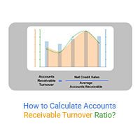
Calculate accounts receivable turnover ratio to measure credit collection speed, improve cash flow, and strengthen your financial strategy. Read on!
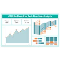
A Customer Relationship Management Dashboard centralizes data, tracks key metrics, and drives smarter business decisions. Discover now!
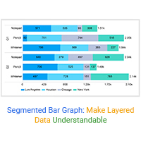
Unlock the power of data with this guide to Segmented Bar Graphs. Learn its types, pros and cons, and when to use it for clear data visualization in Excel.