How to Add Data Bars in Excel for Improved Insights

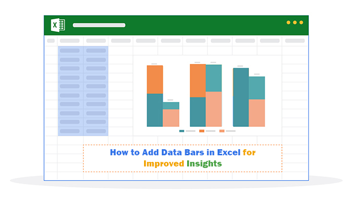
How do I add data bars in Excel? This question often arises when looking for a simple way to make numbers stand out visually. Data bars are a dynamic feature that turns plain cells into visual value indicators. They help you compare data at a glance, saving time and boosting clarity.

Think about this: the average person processes visuals 60,000 times faster than text. In a world where 2.5 quintillion bytes of data are created daily, tools like data bars in Excel are essential. They transform overwhelming rows of numbers into easy-to-read visuals.

How to add data bars in Excel isn’t just about creating colorful cells. It’s about using Excel to communicate better. Imagine tracking sales, grades, or performance metrics—data bars quickly highlight patterns and trends. No more hunting through numbers to find insights.

You can stand out by adding tools like data bars to your toolkit. Professionals who use advanced Excel features are 12% more productive on average. That productivity often translates to better outcomes and recognition.

Whether managing small projects or large datasets, learning to add data bars in Excel can elevate your work. It’s a skill that’s practical, easy to master, and impactful. And the best part? You can start using it today to simplify your data story.

First…

What are Data Bars in Excel?

Definition: Excel data bars are visual tools that turn numbers into bar charts within cells. They show the relative size of values, making data easier to compare. The longer the bar, the higher the value.

These bars are conditional formatting and excellent for creating quick comparisons, much like a side-by-side bar chart. They help highlight patterns, trends, or outliers in your data. You might need to use traditional charting tools for more complex visualizations, such as an Overlapping Bar Chart in Excel. However, data bars offer a simpler, in-cell alternative.

Data bars can be solid or gradient and adjust as values change. This feature saves time and enhances data visualization in spreadsheets.

How to Add Data Bars in Excel?

Bringing data to life is crucial in today’s data-driven world. Excel’s data bars are a simple yet powerful way to visualize numbers and spot trends instantly. Whether working with sales reports, grades, or project metrics, these bars make your spreadsheets more dynamic and readable. Let’s explore how to add data bars in Excel—both with and without displaying values.

How to Add Data Bars with Values

1. Start by entering your data in Excel. Highlight the rows where you want to apply data bars. Before proceeding, ensure you’ve organized your dataset effectively. This step is similar to how to select data for a chart in Excel.
2. Navigate to the “Home” tab, click “Conditional Formatting,” and choose the desired data bar format.

3. Select the “Green Fill” option under “Gradient Fill” styles to make your data visually appealing. Instantly, you’ll see bars representing the values in each cell.

How to Add Data Bars Without Values

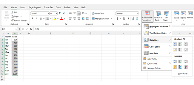
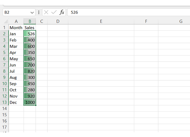
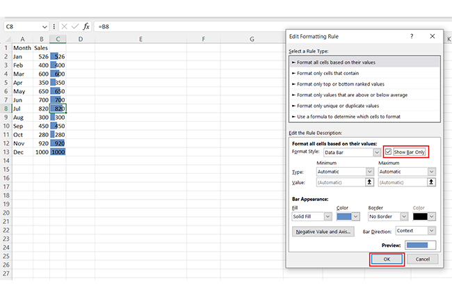
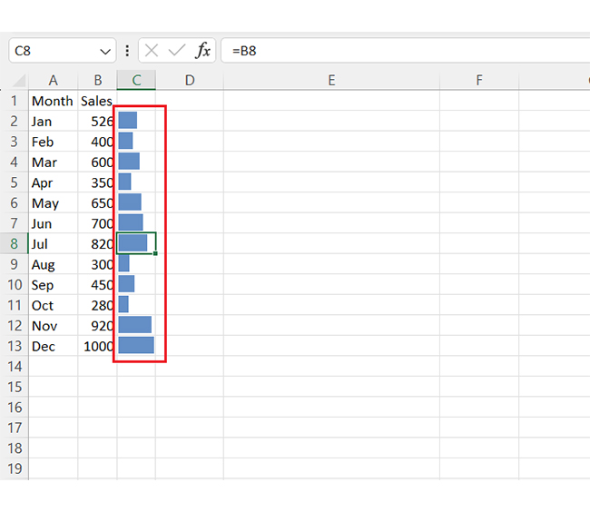
Do you want bars without numbers in the cells? Follow these steps:

1. Add your data to Excel. This is the data for your Excel chart.
2. Copy the data from the cells where you want to base the bars.

3. After applying the format, you can drag the cell to populate the complete set of values as shown below:

4. Paste the data in the desired range and apply the data bar format using “Conditional Formatting”. For clarity, choose “Solid Fill”.

5. Your data will appear as below.

6. Select the range with bars, click “Conditional Formatting”, and go to “Manage Rules”.

7. Click Edit Rules as follows.

8. Check the “Show Bars Only” box and click “OK”.

9. Click the “OK” button again, as shown below:

10. Finally, the bars without values will appear as shown:

Which Data Bar Fill Type Is Better to Choose in Excel?

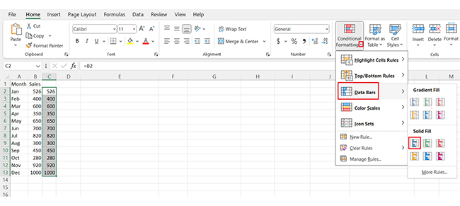
Excel offers two data bar fill types: Gradient Fill and Solid Fill. Choosing the right one depends on your data and presentation needs. Both have unique advantages, but knowing when to use each can make your spreadsheets more effective.

• Gradient Fill: Gradient Fill is ideal for a polished, subtle look. It gradually fades from the bar’s start to its end, creating a sleek, professional appearance. Use Gradient Fill when presenting data to stakeholders or creating reports that need a modern touch. It’s visually appealing and works well for large datasets, ensuring the bars don’t overpower the content.
• Solid Fill: Solid Fill is all about clarity and impact. The bars have bold, uniform colors that stand out instantly. This style is perfect for quick comparisons or when you want your data to grab attention. Solid Fill is also better for smaller datasets where precision and readability matter more than aesthetics.

How to Add Excel Data Bars for Specific Cells?

Want to make your data pop without overwhelming your spreadsheet? Data bars are the perfect way to add instant visual appeal. They’re quick, and easy, and help highlight trends at a glance.

Let’s break it down step by step:

1. Select the cells: Highlight the specific cells where you want to add data bars. Be precise!
2. Open conditional formatting: Navigate to the Home tab and click on Conditional Formatting in the ribbon.
3. Choose data bars: Hover over Data Bars to see gradient and solid fill options. Pick the one that best suits your style.
4. Apply data bars: Click on your desired option. Excel will instantly add data bars to the selected cells.
5. Customize (optional): Want a unique look? Adjust bar colors, and alignments, or choose whether to display values alongside bars.

How to Create Data Bars in Excel?

Data speaks louder when it’s visual. That’s why data visualization is crucial in analysis—it turns boring numbers into insights you can see. Excel’s data bars are a great start, but let’s be honest—the chart elements in Excel are limited.

Do you want stunning visuals that go beyond basic charts? Enter ChartExpo, the ultimate tool for creating engaging, custom visuals. Install ChartExpo and say goodbye to Excel’s constraints and hello to next-level data storytelling.

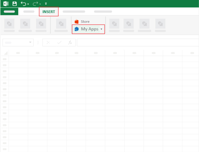
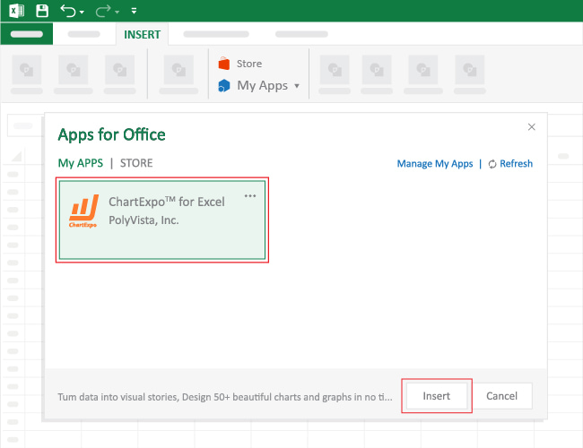
Let’s learn how to install ChartExpo in Excel.

1. Open your Excel application.
2. Open the worksheet and click the “Insert” menu.
3. You’ll see the “My Apps” option.
4. In the Office Add-ins window, click “Store” and search for ChartExpo on my Apps Store.
5. Click the “Add” button to install ChartExpo in your Excel.

ChartExpo charts are available both in Google Sheets and Microsoft Excel. Please use the following CTAs to install the tool of your choice and create beautiful visualizations with a few clicks in your favorite tool.

Example

Let’s analyze this sample data with a dynamic graph in Excel using ChartExpo.

Channel	Gender	Views	Clicks	Sales
Facebook	Male	15000	1000	55
Facebook	Female	4000	150	10
Google	Male	9000	1200	60
Google	Female	3000	325	15
X (Twitter)	Male	7000	900	33
X (Twitter)	Female	2000	125	20

• To get started with ChartExpo, install ChartExpo in Excel.
• Now Click on My Apps from the INSERT menu.

• Choose ChartExpo from My Apps, then click Insert.

• Once it loads, scroll through the charts list to locate and choose the “Clustered Stacked Bar Chart”. This chart is best suited to this scenario.

• You will see a Clustered Stacked Bar Chart on the screen.

• Click the “Create Chart From Selection” button after selecting the data from the sheet, as shown.

• ChartExpo will generate the visualization below for you.

• If you want to have the chart’s title, click Edit Chart, as shown in the above image.
• Click the pencil icon next to the Chart Header to change the title.
• It will open the properties dialog. Under the Text section, you can add a heading in Line 1 and enable Show.
• Give the appropriate title of your chart and click the Apply button.

• You can change the color of the Male section by clicking on the Legend small pencil icon:

• You can change the color of the Female section by clicking on the Legend small pencil icon:

• Click the “Save Changes” button to persist the changes.

• Your Clustered Stacked Bar Chart will appear as below.

Insights

• • Male users outperform females with higher views, clicks, and sales across all channels.

• Google excels in sales. It dominates sales performance, especially among male users.
• Facebook achieves the highest overall views but has lower sales efficiency.

How to Use Data Bars in Microsoft Excel for Enhanced Chart Visualization:

1. Open your Excel Application.
2. Install ChartExpo Add-in for Excel from Microsoft AppSource to create interactive visualizations.
3. Select the Clustered Stacked Bar Chart from the list of charts.
4. Select your data.
5. Click on the “Create Chart from Selection” button.
6. Customize your chart properties to add header, axis, legends, and other required information.

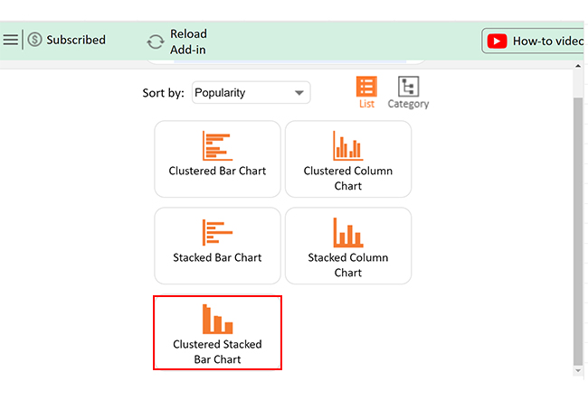
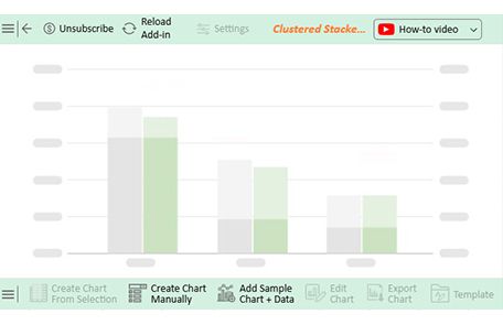
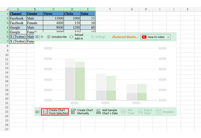
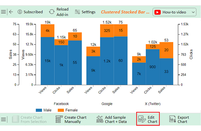
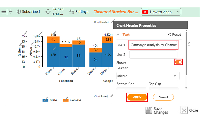
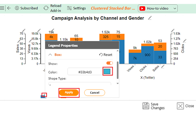
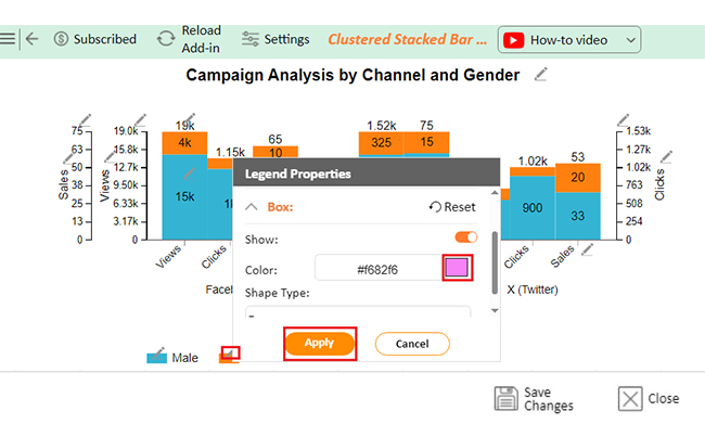
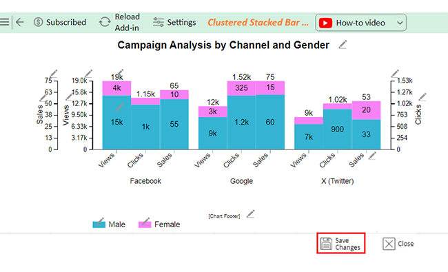
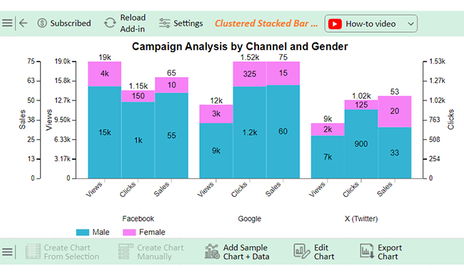
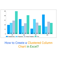
The following video will help you create a Clustered Stacked Bar Chart in Microsoft Excel.

FAQs

How can you access the data bars menu in Excel?

To access the data bars menu in Excel, follow these steps:

1. Select the cell range.
2. Go to the Home tab.
3. Click on Conditional Formatting.
4. Choose Data Bars from the dropdown menu.
5. Pick a style.

How do I add a data bar in an Excel cell?

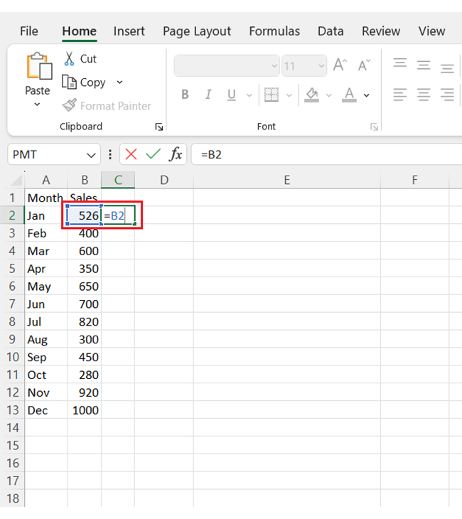
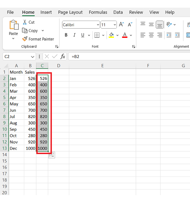
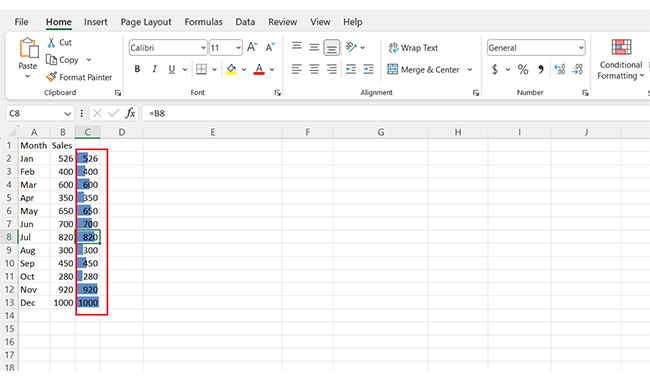
To add a data bar in an Excel cell:

1. Select the desired cell.
2. Navigate to the Home tab.
3. Click Conditional Formatting.
4. Choose Data Bars.
5. Select a preferred style.

How to use conditional formatting to create data bars in Excel?

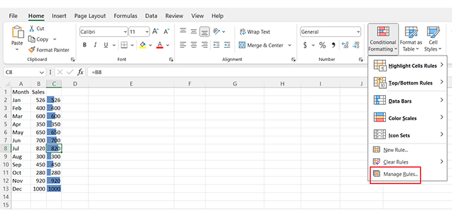
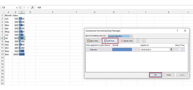
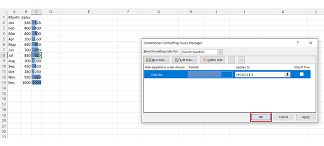
To create data bars using conditional formatting in Excel:

1. Highlight the data range.
2. Click the Home tab.
3. Select Conditional Formatting.
4. Choose Data Bars.
5. Pick a gradient or solid color style.

Wrap Up

Adding data bars in Excel is a powerful way to enhance data visualization. They simplify large datasets, like a Progress Bar Chart, offering instant insights into completion or performance. With just a few clicks, you can create a visual impact that improves clarity.

This feature is ideal for comparing values within a range. It highlights trends and outliers, bringing focus to critical data points. Whether for reports or presentations, it ensures your audience grasps the data quickly.

Customizing data bars is simple, too. You can adjust colors, directions, and rules to suit your needs. These options allow you to match the bars to your Data for Excel Chart, ensuring a cohesive and meaningful design.

When using data bars, avoid clutter. Stick to clean and meaningful visuals. Too many bars or colors can confuse your audience – aim for simplicity and focus.

Data bars work seamlessly with other Excel features. Combine them with conditional formatting, filters, or pivot tables. This integration makes them versatile and efficient. For Radial Bar Charts or advanced visuals, data bars offer foundational insights before exploring complex representations.

Now you know how to add data bars in Excel. Use them to transform raw numbers into engaging visuals. Try this feature today with ChartExpo and bring your spreadsheets to life.