Amortization Schedule in Excel: A Complete Guide

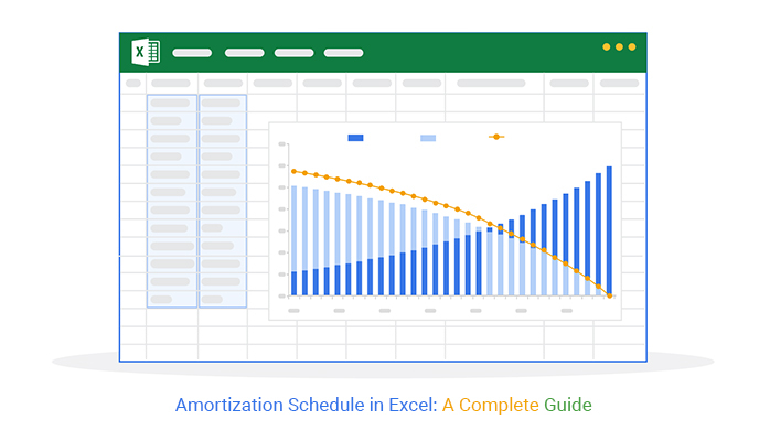
What is an amortization schedule in Excel?

You’ve come across this tool if you’re managing loans or payments. An amortization schedule breaks down your loan payments into principal and interest over time. Creating one that automatically calculates these payments in Excel helps you stay on track easily.

An amortization schedule in Excel saves you time and effort, simplifying financial planning. For instance, the average American household carries nearly $150,000 in debt. These include mortgages, car loans, and student loans. With such high numbers, keeping track of payments is crucial. Excel’s built-in functions help you visualize the following: how much you owe each month, how much interest you pay, and when your loan will be paid off.

Amortization schedules in Excel aren’t just for large loans—small businesses also use them to manage their finances. Nearly 30% of small businesses in the U.S. use spreadsheets for financial management.

Let’s see how you can set up an amortization schedule in Excel and make it work for you.

Table of Contents:

1. What is an Amortization Schedule in Excel?
2. Why is a Loan Amortization Schedule in Excel Useful?
3. What are the Loan Amortization Schedule Functions in Excel?
4. How to Create an Amortization Schedule in Excel?
5. Who Can Use an Amortization Schedule?
6. How to Make a Loan Amortization Schedule in Excel with Extra Payments?
7. How to Analyze Amortization Schedule in Excel?
8. Wrap Up

First…

What is an Amortization Schedule in Excel?

Definition: An amortization schedule is a tool for tracking loan payments over time. It shows how much of each payment goes toward interest and how much goes toward the principal balance.

Excel automatically calculates these values using built-in functions. This makes it easier to plan payments and see how a loan will be paid off. Whether for personal or business loans, an amortization schedule in Excel provides clear, organized financial tracking for data-driven decision-making.

Why is a Loan Amortization Schedule in Excel Useful?

Managing a loan can be overwhelming, but Excel makes it simpler. Here’s how:

• Payment breakdown: You can see exactly how much of each payment goes toward the interest and how much goes toward the principal. This helps you track your progress and plan accordingly.
• Financial planning: Planning your finances is easier when you can predict your payments. Excel’s schedule gives you a clear picture of when your loan will be paid off and how much you’ll owe each month.
• Cost analysis: Do you want to know how much interest you’re paying over the life of the loan? An amortization schedule in Excel helps you understand the true cost of your loan.
• Scenario comparison: You can compare different loan terms or interest rates by adjusting the numbers in your schedule. This helps you choose the best option for your situation.
• Customizability: Excel allows you to customize your schedule. Whether it’s adjusting payment dates or adding extra payments, you can tweak it to fit your needs.

What are the Loan Amortization Schedule Functions in Excel?

When creating a loan amortization schedule in Excel, several powerful functions help make it all come together. These functions simplify the process and ensure accuracy. Let’s explore the key functions:

• PMT (Payment Function): It calculates the fixed monthly payment for a loan based on the interest rate, loan term, and loan amount. This is the starting point for your schedule.
• IPMT (Interest Payment): IPMT helps you break down that amount, giving you a clearer view of your loan payments.
• PPMT (Principal Payment): It shows how much of each payment goes toward the principal balance. This helps you track how your debt decreases over time.
• FV (Future Value): This function calculates the remaining balance after a certain number of payments. It’s useful when you want to see your loan balance.
• RATE (Interest Rate): RATE helps you determine the interest rate for your loan based on payments, loan amount, and term. It’s a handy tool if you’re unsure about your loan’s interest rate.
• NPER (Number of Periods): It calculates how long (months or years) it will take to pay off the loan. It bases the calculation on your payment amount, interest rate, and loan value.

How to Create an Amortization Schedule in Excel?

Creating an amortization schedule in Excel helps you track loan payments, interest, and principal over time. In case you’re planning a mortgage, auto loan, or any installment payment, having a clear breakdown can be helpful. Let’s walk through the steps;

1. Add Your Data

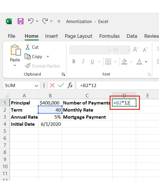
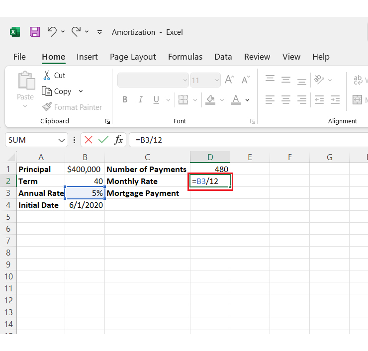
Start by entering your loan details into the Excel sheet. Here’s what you’ll need:

• • Loan Amount (Principal)
  • Annual Interest Rate
  • Loan Term (in years)
  • Number of Payments (Total payments)

2. Set the Monthly Interest Rate

• • To find the monthly interest rate, simply divide your annual rate by 12. In Excel, you can enter this formula:
  • Annual Interest Rate / 12

3. Use the Amortization Schedule Function, such as the PMT:

Who Can Use an Amortization Schedule?

An amortization schedule is a powerful tool that different groups of people can use. It breaks down loan payments to show how much of each payment goes toward interest and how much goes toward the principal. Let’s see who can benefit from an amortization schedule.

• Borrowers: If you’re taking out a loan it shows how much you’ll pay each month, including the interest and principal. It’s helpful for budgeting and understanding how long it will take to pay off your debt.
• Lenders and financial institutions: Lenders use amortization schedules to manage their risk and track the repayment process. These schedules assist in analyzing cash flow, forecasting future income, and ensuring borrowers meet their payment obligations on time.
• Financial advisors and accountants: They use it to provide insights into the cost of borrowing and help with repayment strategies. By reviewing the schedule, they can advise clients on how to pay off loans more efficiently.
• Businesses: An amortization schedule is critical for managing cash flow and understanding how debt will impact the company’s finances over time. It also helps with tax planning and financial reporting.
• Educators and students: Amortization Schedule is used to teach the principles of loan repayment, the time value of money, and financial planning. Students get a hands-on way to learn how loans work in the real world.

How to Make a Loan Amortization Schedule in Excel with Extra Payments?

Want to speed up your loan payoff? Adding extra payments in Excel helps you save money on interest and pay off your loan. Here’s how to do it step by step.

1. Input loan details: First, set up your loan inputs. For example:

• • Loan Amount: $10,000
  • Annual Interest Rate: 5%
  • Loan Term: 5 years
  • Extra Payment: $50

2. Setup the schedule table: Create a table with the following columns:

• • Period
  • Payment
  • Extra Payment
  • Total Payment
  • Interest
  • Principal
  • Remaining Balance

3. Calculate fixed monthly payment: Use the PMT function to determine the fixed monthly payment. The formula is: =PMT(Annual Interest Rate/12, Loan Term×12, -Loan Amount)

4. Populate the table:

• • Period (Column A): List the payment periods (1, 2, 3, etc.).
  • Interest (Column E): Calculate the interest for the current balance using:
  • =Remaining Balance × (Annual Interest Rate / 12)
  • Principal (Column F): Subtract the interest from the total payment:
  • =Payment – Interest
  • Extra Payment (Column C): Enter the extra payment amount you want to apply.
  • Total Payment (Column D): Add the regular and extra payments:
  • =Payment + Extra Payment
  • Remaining Balance (Column G): Subtract the principal and extra payment from the previous balance:
  • =Previous Balance – Principal – Extra Payment

5. Copy formulas down: Drag the formulas down through the table until the loan balance reaches zero. Adjust the final payment if needed.
6. Add summary section: Calculate the total interest paid and how much you’ve saved by making extra payments.

How to Analyze Amortization Schedule in Excel?

Excel is a great tool for calculations, but it often falls short when it comes to data visualization. It can handle numbers, but it’s not always the best at showing them in an easy-to-digest way.

An amortization schedule in Excel comes in handy for tracking loan payments. However, when it comes to creating clear, insightful visualizations, understanding the types of charts and graphs Excel offers can help you go beyond its basic features for more impactful representations.

Enter ChartExpo, the solution to Excel’s data visualization limitations. With it, you can turn complex financial data into visually appealing, easy-to-understand charts.

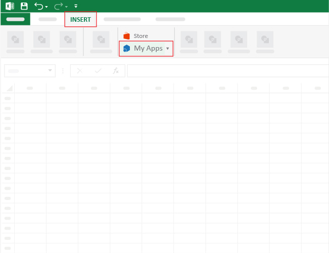
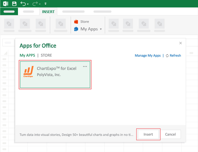
Let’s learn how to install ChartExpo in Excel.

1. Open your Excel application.
2. Open the worksheet and click the “Insert” menu.
3. You’ll see the “My Apps” option.
4. In the Office Add-ins window, click “Store” and search for ChartExpo on my Apps Store.
5. Click the “Add” button to install ChartExpo in your Excel.

ChartExpo charts are available both in Google Sheets and Microsoft Excel. Please use the following CTAs to install the tool of your choice and create beautiful visualizations with a few clicks in your favorite tool.

Example

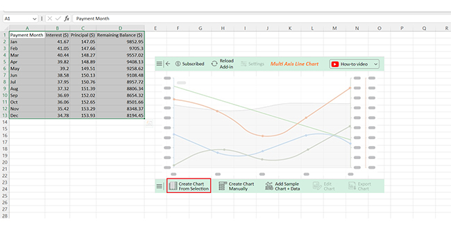
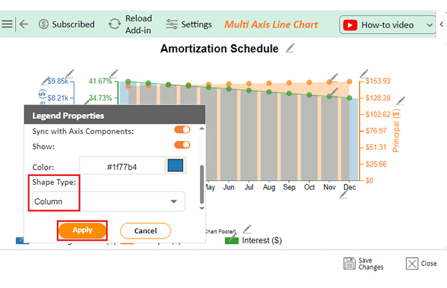
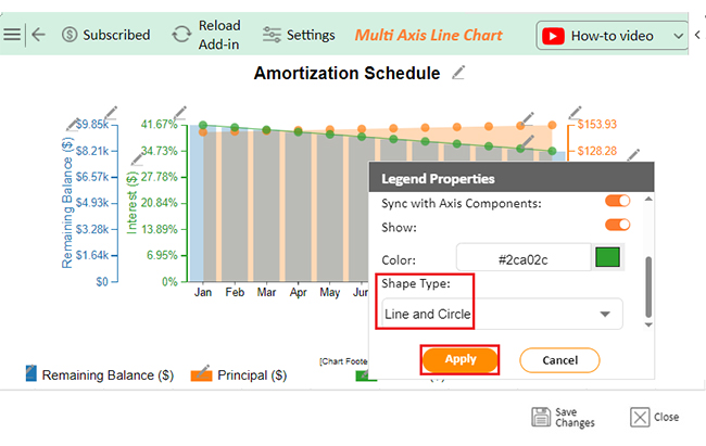
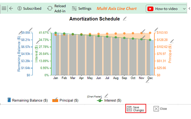
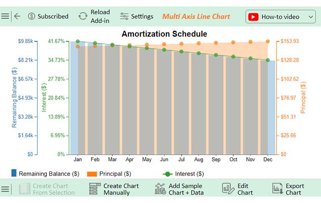
Let’s analyze this Amortization schedule sample data in Excel using ChartExpo.

Payment Month	Interest ($)	Principal ($)	Remaining Balance ($)
Jan	41.67	147.05	9,852.95
Feb	41.05	147.66	9,705.30
Mar	40.44	148.27	9,557.02
Apr	39.82	148.89	9,408.13
May	39.2	149.51	9,258.62
Jun	38.58	150.13	9,108.48
Jul	37.95	150.76	8,957.72
Aug	37.32	151.39	8,806.34
Sep	36.69	152.02	8,654.32
Oct	36.06	152.65	8,501.66
Nov	35.42	153.29	8,348.37
Dec	34.78	153.93	8,194.45

• To get started with ChartExpo, install ChartExpo in Excel.
• Now Click on My Apps from the INSERT menu.

• Choose ChartExpo from My Apps, then click Insert.

• Once it loads, scroll through the charts list to locate and choose the “Multi Axis Line Chart”.

• After clicking on the chart, you will see the Multi Axis Line Chart on the screen.

• Click the “Create Chart From Selection” button after selecting the data from the sheet, as shown.

• ChartExpo will generate the visualization below for you.

• You can change the Data Representation as follows:

• If you want to have the chart’s title, click Edit Chart.

• Click the pencil icon next to the Chart Header to change the title.
• It will open the properties dialog. Under the Text section, you can add a heading in Line 1 and enable Show.
• Give the appropriate title of your chart and click the Apply button.

• You can add the dollar sign with “Principal” as follows:

• You can add the percentage sign with “Interest” as follows:

• You can add the dollar sign with “Remaining Balance” as follows:

• You can enable the Legend Show button as follows:

• Change the Legend shape of “Remaining Balance” to Column and click the “Apply” button.

• Change the Legend shape of “Interest” into a Line and Circle and click the “Apply” button.

• Click the “Save Changes” button to persist the changes made to the chart.

• Your final Multi Axis Line Chart will look like the one below.

Insights

• Monthly loan payments show a pattern of declining interest and increasing principal contributions.
• The loan balance decreases consistently over 12 months. By December, the remaining balance drops from $9,852.95 to $8,194.45.
• These trends reflect steady repayment progress throughout the year.

Simplify Amortization Schedule in Microsoft Excel:

1. Open your Excel Application.
2. Install ChartExpo Add-in for Excel from Microsoft AppSource to create interactive visualizations.
3. Select the Multi-Axis Line Chart from the list of charts.
4. Select your data.
5. Click on the “Create Chart from Selection” button.
6. Customize your chart properties to add header, axis, legends, and other required information.

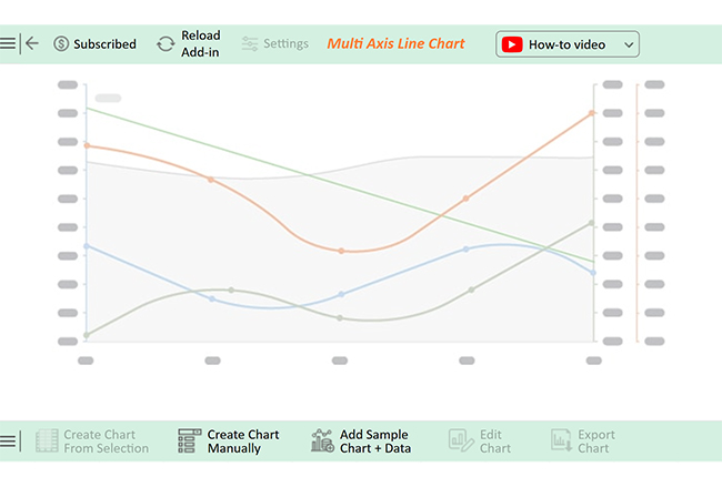
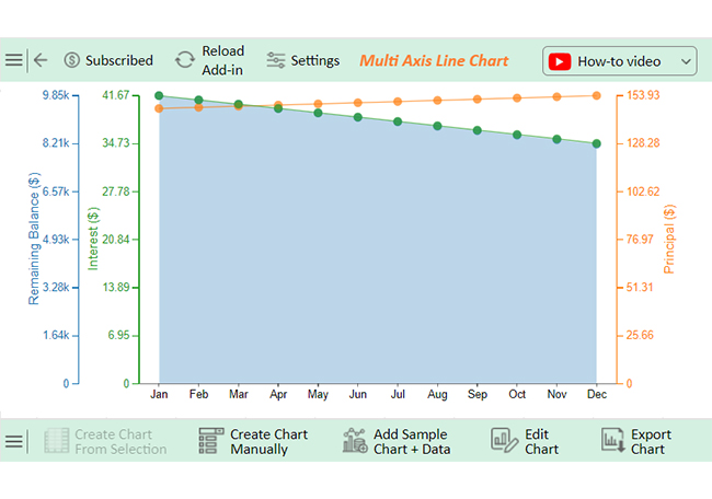
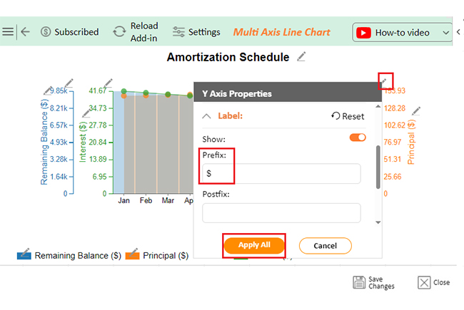
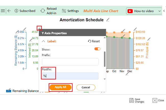
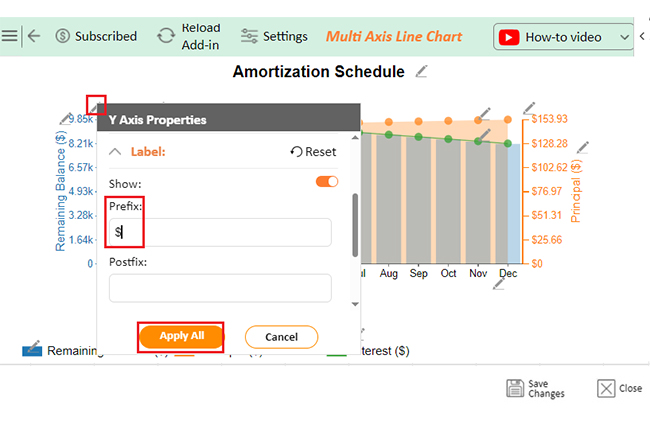
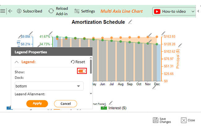
The following video will help you create a Multi-Axis Line Chart in Microsoft Excel.

FAQs

How do you get an amortization schedule in Excel?

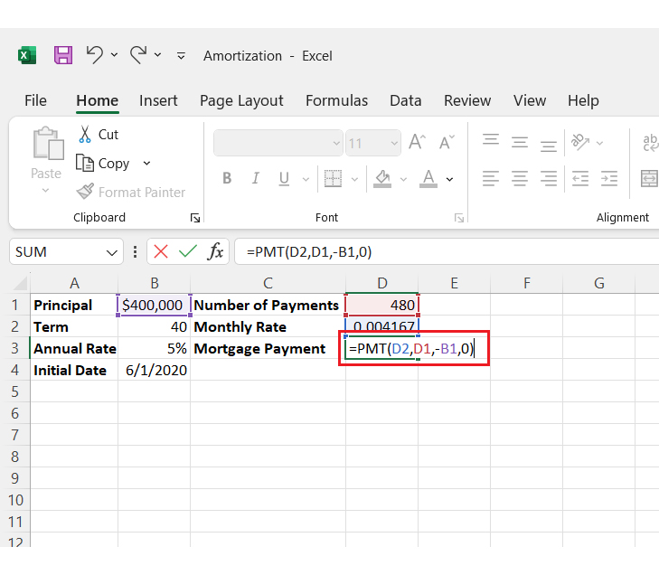
Use the PMT function to calculate monthly payments. Then, create columns for period, interest, principal, and remaining balance. Apply formulas to calculate interest and principal and adjust the balance over time.

Which Excel function is most important when creating an amortization schedule?

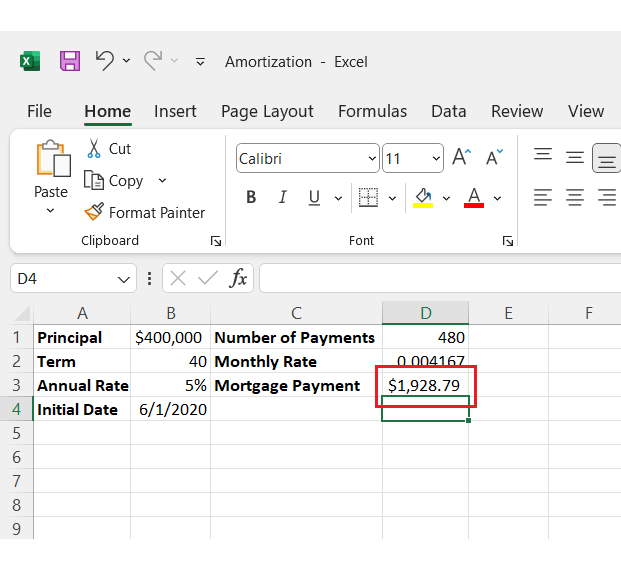
PTM is an important Excel function for creating an amortization schedule. It calculates the fixed monthly payment based on loan amount, interest rate, and term. This is essential for determining consistent payments throughout the loan’s life.

Wrap Up

An amortization schedule in Excel is a powerful tool for managing loans. It helps you break down monthly payments into interest and principal. Thus, using Excel, you can easily track your loan progress over time.

The PMT function key calculates the fixed monthly payment, which is the foundation of the entire schedule. Once the payment is established, other functions like IPMT and PPMT help you calculate interest and principal amounts for each period.

Creating an amortization schedule lets you see how extra payments impact your loan. You can visualize the progress of your loan and adjust payments as needed. This helps you pay off debt faster and save on interest.

It’s easy to customize the schedule with Excel. Whether for a mortgage, car loan, or business loan, you can tailor it to your needs. Moreover, you can add extra payments and see how they affect the remaining balance.

Incorporating charts and graphs into your amortization schedule further enhances its usefulness. Data visualization makes it easier to understand trends and track progress toward loan payoff.

Conclusively, an amortization schedule in Excel is a valuable tool for anyone managing a loan. It helps keep your payments organized and clarifies the financial path ahead.