Categories
Few Excel formulas pack as much analytical power into a single expression as SUMPRODUCT. Knowing how to use SUMPRODUCT in Excel lets you multiply paired values across ranges, evaluate multiple conditions, and return a combined total in one step, all without building out extra helper columns or nesting several functions together.
This guide walks through the syntax, real-world examples, and proven techniques that make this formula valuable across financial analysis, performance tracking, and reporting workflows.
Whether you work with small datasets or large structured tables, the steps covered here will help you apply this formula with confidence and get accurate results every time.
Definition: To understand how to use SUMPRODUCT in Excel, start with what it does: this formula takes two or more arrays, multiplies the values at each corresponding position, and returns the sum of all those products.
Rather than treating a range as a single block, it processes every row or column pair individually, making it well-suited for totaling paired data such as unit quantities and prices.
Professionals applying how to use SUMPRODUCT in Excel rely on it for weighted averages, conditional totals, and multi-criteria performance summaries. Unlike SUM or COUNT, it can assess several conditions at once within a single expression.
A frequent source of errors is supplying arrays of unequal length, so always confirm that every range covers the same number of cells before running the formula.
Knowing how to use SUMPRODUCT in Excel removes the need to build long nested expressions for routine analytical tasks. It keeps formulas compact and spreadsheets easier to manage.
Here is why analysts and professionals rely on it:
Seeing where this formula fits in practice makes it far easier to apply correctly. Knowing how to use SUMPRODUCT in Excel opens up tasks ranging from basic array math to conditional reporting across multiple criteria.
Common applications include:
Grasping the syntax is the first step toward applying this formula reliably across any dataset. Knowing how to use SUMPRODUCT in Excel across different scenarios becomes simpler once you understand its underlying structure, especially when working with organized data prepared through how to use Excel Power Query.
=SUMPRODUCT(array1, [array2], [array3], …)
The first array argument is required; all additional arrays are optional. The formula multiplies the values at each matching position across all supplied arrays and then adds those products.
Every array must share identical dimensions, meaning the same number of rows and columns. When dimensions differ, the formula returns an error. You can also embed logical expressions inside the arrays to perform conditional calculations without a separate column.
Working through concrete examples is the clearest way to understand how to use SUMPRODUCT in Excel across different analytical scenarios.
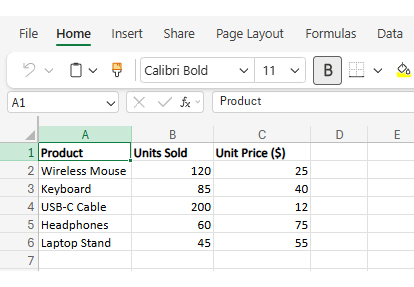
Consider a retail store that tracks weekly product sales:
Input the number of units sold for each product.
Add the selling price per unit for each product.
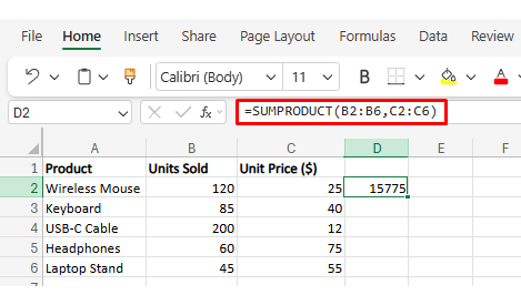
Type = SUMPRODUCT (B2:B6, C2:C6) to multiply units by prices and sum the totals automatically.
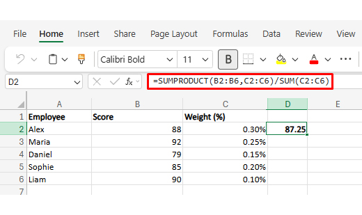
Consider a company that evaluates employee performance using weighted KPIs:
Add each employee’s performance rating.
Convert percentages into decimals (0.30, 0.25, etc.).
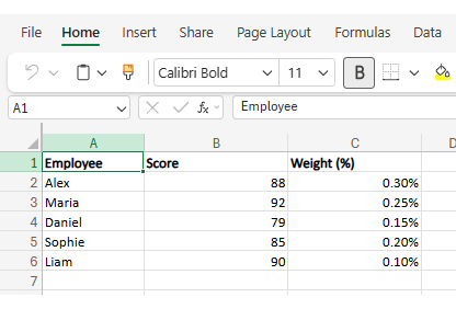
Use = SUMPRODUCT (B2:B6, C2:C6) / SUM(C2:C6) to multiply scores by weights and divide by total weight.
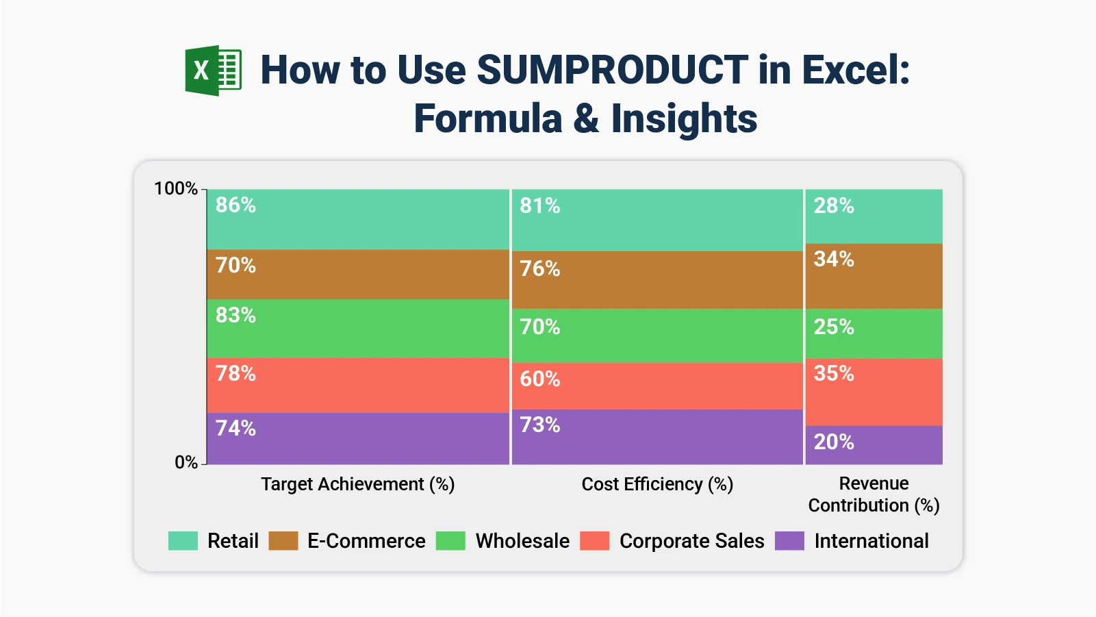
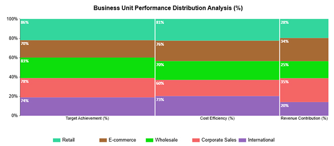
In the Business Unit Performance Distribution Analysis, Retail delivers the strongest metric balance, while Corporate Sales and E-commerce account for the largest shares of revenue contribution.

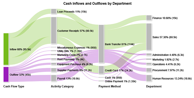
The Cash Inflows and Outflows by Department chart maps cash movement across activities and payment channels, making each department’s proportional allocation and contribution visible at a glance.
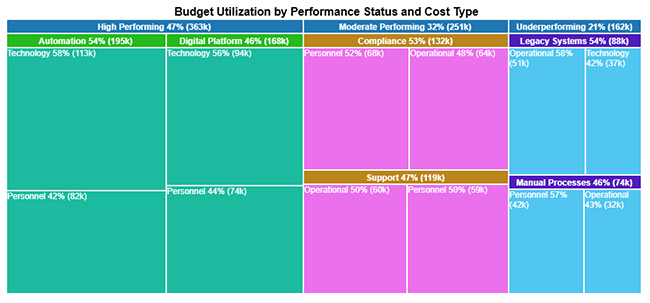
The Budget Utilization by Performance Status and Cost Type view reveals how budget amounts are distributed proportionally across performance levels and cost categories, capturing both the weighted and conditional dimensions of financial resource planning.
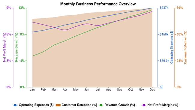
The Monthly Business Performance Overview tracks revenue growth, profit margin, operating expenses, and customer retention to give a complete picture of business health over time.
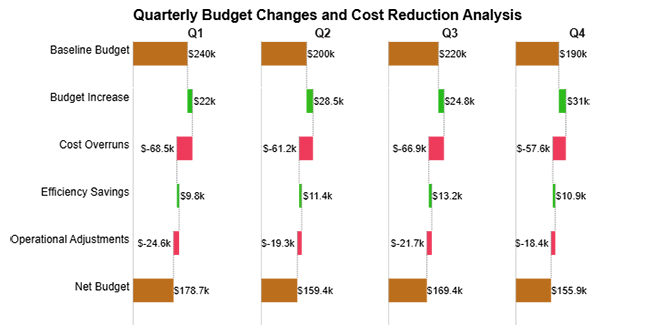
The Quarterly Budget Changes and Cost Reduction Analysis charts how periodic gains and losses stack up to shape overall financial outcomes across each quarter.
Analyzing SUMPRODUCT results in Excel helps you evaluate weighted data, compare multiple variables, and uncover deeper insights from complex datasets. Follow these steps to effectively interpret your results:
Start by reviewing the data used in the SUMPRODUCT formula. Ensure your arrays or ranges are aligned correctly, as SUMPRODUCT multiplies corresponding values and then sums them. A clear structure is essential for accurate analysis.
Use the SUMPRODUCT function to calculate weighted totals or combined results across multiple ranges. This is especially useful for analyzing performance metrics, costs, or contributions across different categories.
Instead of looking at a single total, analyze how each variable contributes to the final result. Separate your data into categories such as departments, products, or regions to better understand the impact of each component.
Use additional formulas or pivot tables to compare SUMPRODUCT results across different segments. This helps identify which categories perform better and where improvements are needed.
Convert your results into charts like comparison bars or stacked visuals to make insights easier to interpret. For more advanced and interactive charts, you can use ChartExpo to simplify complex data visualization.
Analyze the visual output to identify patterns, variations, and performance differences. Focus on how different segments contribute to overall results and where optimization opportunities exist.
Include a final visualization, such as a stacked comparison chart, that highlights how different business units contribute to key metrics, including target achievement, cost efficiency, and revenue contribution. This type of chart makes it easy to compare performance across multiple categories and clearly communicate insights.
Choosing to learn how to use SUMPRODUCT in Excel delivers real gains in everyday spreadsheet tasks. Below are the core advantages that come with regular use.
Core advantages include:
Consistent habits eliminate the most common sources of error. These practices will sharpen your understanding of how to use SUMPRODUCT in Excel and keep results reliable.
One practical application of how to use SUMPRODUCT in Excel: enter each score in one column and its corresponding weight in another, nest both ranges inside the formula, and divide the result by the total of the weights column. Each value then contributes proportionally to the final figure.
The most common causes are ranges of different lengths, text values mixed into numeric columns, or parentheses placed in the wrong position within a logical condition. Checking that all arrays share identical dimensions and that numeric ranges contain no text will resolve most issues.
Add a logical test inside the formula that compares each row’s location field against your target value, then multiply the resulting TRUE/FALSE array by the fee column. SUMPRODUCT sums only the matching rows, giving you a location-specific total without any helper columns.
Knowing how to use SUMPRODUCT in Excel transforms the way you approach multi-condition analysis. This formula compresses tasks that would normally require multiple helper columns or deeply nested structures into a single, readable expression, giving you faster results and fewer opportunities for error across every project you tackle.
Pair the formula with strong visualization practices, and your outputs become not just accurate but genuinely useful to decision-makers and stakeholders. Start with the examples in this guide, apply them to your own datasets, and build on each technique until working with this formula feels as natural as any other tool in your analytical toolkit.
How much did you enjoy this article?


Explore 15 best financial charts to track revenue, costs, and profits, simplifying analysis and helping businesses make smarter financial decisions.

Learn cross tabulation in Excel to analyze data, identify patterns, and uncover relationships using Pivot Tables for better insights and reporting.

Learn how to add and customize trendlines in Excel to uncover insights, track patterns, and predict future data points.