Categories
What is the weighted average in Excel? This powerful calculation method transforms how we analyze data in spreadsheets. It goes beyond simple averages, considering the importance of each value.
Imagine grading a class where some assignments matter more than others. That’s where weighted averages shine. They allow you to assign different levels of importance to various data points.
The Excel weighted average function isn’t limited to academics. Investment firms use it to calculate portfolio returns. HR departments apply it to employee performance evaluations. And even weather forecasters utilize weighted averages to predict temperatures.
Let’s talk numbers. A study found that weighted average Excel can improve forecast accuracy by up to 25%. That’s a significant boost in predictive power. Moreover, 65% of data analysts report more reliable results when incorporating weighted averages in their Excel models.
Weighted averages on Excel also enhance decision-making processes. Assigning appropriate weights helps businesses prioritize factors in complex scenarios. This leads to more informed choices and better outcomes.
Follow through as we delve into the process of calculating and utilizing weighted averages. This blog post will enhance your ability to analyze and make decisions.
First…
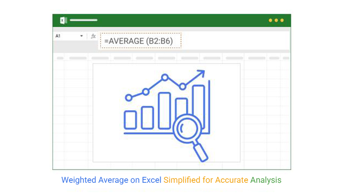
Definition: The weighted average in Excel calculates the mean of values, giving weights to each value. Unlike a simple average, it accounts for the significance of each number.
To calculate the weighted average in Excel:
This method is useful for handling data where some elements are more important than others.
Calculating a weighted average in Excel goes beyond crunching numbers; it’s about making data-driven decisions. When data points don’t carry equal weight, this method gives a more nuanced view of the dataset.
Here’s why it matters:
Here is the weighted average formula in Excel:

where xi is the numerical value of a response and fi is its frequency.
Calculating weighted averages in Excel allows you to find an average where some values contribute more than others. This is useful when dealing with data that has varying levels of importance.
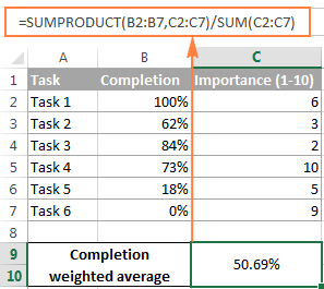
By multiplying each value by its assigned weight and then dividing the sum of those products by the total of the weights, you can easily calculate a weighted average using Excel’s SUMPRODUCT and SUM functions.
Calculating a weighted average in Excel using the SUMPRODUCT function is quick and easy. It’s perfect when some data points matter more than others, like in sales performance or student grading.
Here’s a simple step-by-step guide to get you started:
To calculate a weighted average using the SUM function in Excel or similar tools, follow these steps:
For example, if you have values in column A and weights in column B, create a formula in a new column: =A1*B1.
Use =SUM(C1:Cn) if your weighted values are in column C.
Use =SUM(B1:Bn) if your weights are in column B.
Weighted Average Formula: Weighted Average = SUM(Weighted Values) / SUM(Weights).
Example: If your values are 10, 20, 30 with weights 1, 2, 3:
Weighted Sum = (10×1) + (20×2) + (30×3) = 140
Total Weights = 1 + 2 + 3 = 6
Weighted Average = 140 / 6 = 23.33
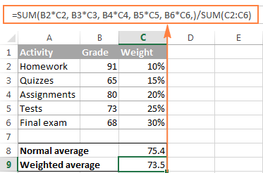
Here iyou know weighted average Excel example belwo:
You have a table showing the grades of students and the corresponding weight (importance) of each assignment in determining the final grade.
| Assignment | Grade | Weight |
| Assignment 1 | 85 | 20% |
| Assignment 2 | 90 | 30% |
| Assignment 3 | 80 | 50% |
Enter the data in Excel:
Convert weights to decimals (if necessary):
Multiply Grades by Weights:
Sum the Weighted Values:
Use the SUM function to add the weighted values: =SUM(D2:D4)
Data analysts, unite! Your spreadsheets are calling.
Today’s hot topic? Weighted averages in Excel – it’s like regular averages but with a dash of favoritism.
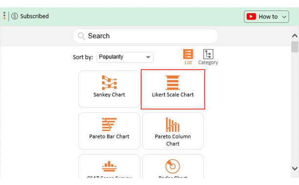
We’ll use a Likert Scale Chart in Excel to visualize and analyze weighted averages in Excel.
Why the Likert Scale Chart?
The connection between weighted averages and Likert scale data lies in how we summarize and interpret survey responses. Likert scales typically feature ordinal data, such as a 1-5 scale. Here, 1 might indicate “Strongly Disagree”, and 5 indicates “Strongly Agree”. Even though this data is ordinal (showing ranks), calculating weighted averages helps extract useful insights.
Here’s how it works:
where xi is the numerical value of a response and fi is its frequency.
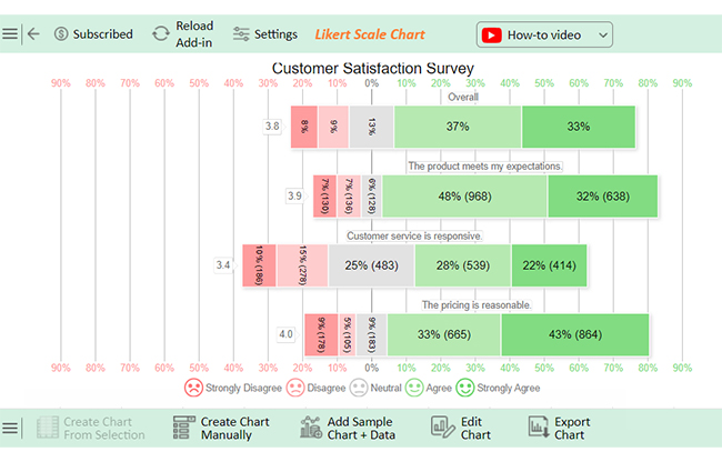
This is where ChartExpo, the superhero of data visualization, comes into play. ChartExpo turns those boring spreadsheets into eye-catching masterpieces that even your boss will understand.
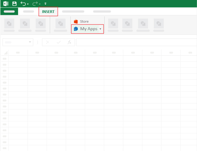
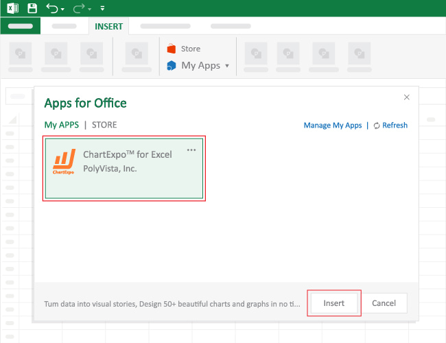
Let’s learn how to install ChartExpo in Excel.
ChartExpo charts are available both in Google Sheets and Microsoft Excel. Please use the following CTAs to install the tool of your choice and create beautiful visualizations with a few clicks in your favorite tool.
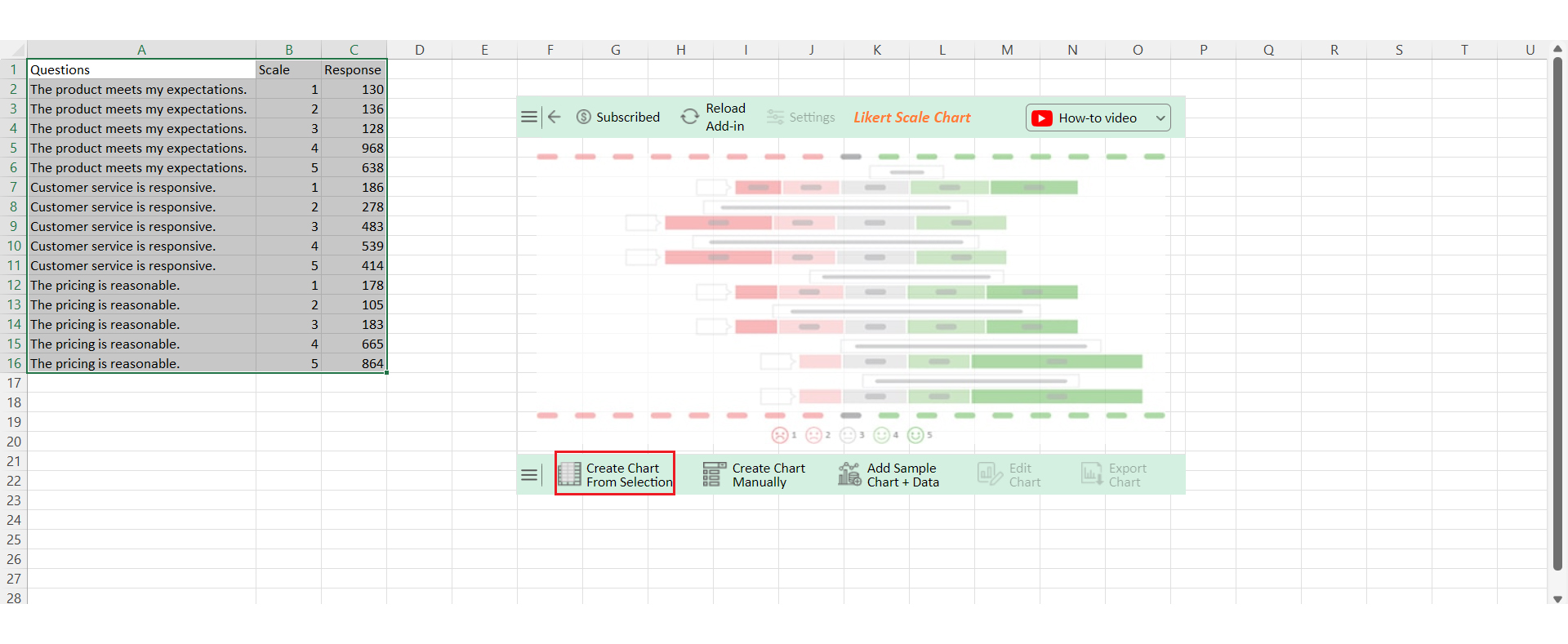
Let’s visualize the weighted average example data below in Excel using ChartExpo and glean valuable insights.
| Questions | Scale | Response |
| The product meets my expectations. | 1 | 130 |
| The product meets my expectations. | 2 | 136 |
| The product meets my expectations. | 3 | 128 |
| The product meets my expectations. | 4 | 968 |
| The product meets my expectations. | 5 | 638 |
| Customer service is responsive. | 1 | 186 |
| Customer service is responsive. | 2 | 278 |
| Customer service is responsive. | 3 | 483 |
| Customer service is responsive. | 4 | 539 |
| Customer service is responsive. | 5 | 414 |
| The pricing is reasonable. | 1 | 178 |
| The pricing is reasonable. | 2 | 105 |
| The pricing is reasonable. | 3 | 183 |
| The pricing is reasonable. | 4 | 665 |
| The pricing is reasonable. | 5 | 864 |
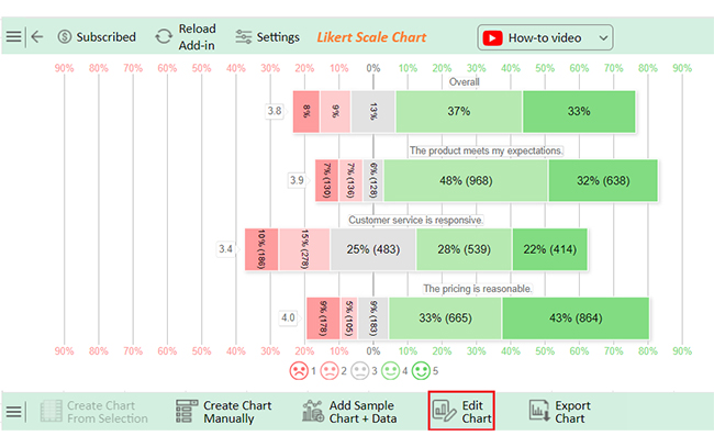
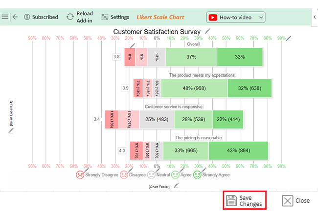
Feedback covers three aspects:
Ratings are based on a scale of 1-5.
Key insights from the data include:
Using Excel templates for weighted averages can save you time. But knowing a few tips will make the process even smoother. Here are some tricks to help you get the most out of your templates:
Yes, you can. First, compute the weighted average using =SUMPRODUCT(values, weights)/SUM(weights). Once calculated, insert a suitable chart (like a line, bar, or scatter plot). This chart can help compare the weighted average with other data points.
Start by calculating the weighted average in Excel or Power BI itself using DAX. Once calculated, you can visualize it through charts like line or bar charts. How? By importing the Excel data or creating a measure in Power BI. This allows for dynamic interaction within the dashboard.
Calculate each data set’s weighted average using the formula =SUMPRODUCT(values, weights)/SUM(weights) for each set. Then, plot these on a bar chart or line graph. This visual will help compare trends or differences across the data sets, highlighting patterns or shifts.
Weighted averages in Excel are essential for analyzing data where different values carry unequal importance. They help you go beyond simple averages by factoring in the significance of each data point. This method is useful in many fields, from finance to grading systems.
Calculating weighted averages involves multiplying each value by its weight. Then, you sum up the products and divide them by the total of the weights. Excel’s SUMPRODUCT and SUM functions make this process easy and efficient.
The advantage of using weighted averages is that they reflect the true importance of each data point. This is especially helpful when dealing with real-world data, where certain values matter more than others.
You can also use weighted averages to make better decisions. Whether you’re analyzing sales, performance metrics, or survey results, this method provides clearer insights. It helps in evaluating situations more accurately.
Weighted averages are commonly used in business and finance to assess investment portfolios or budgets. They help highlight key factors without distorting the overall picture.
Do not hesitate.
Learn how to apply weighted averages in Excel today. It will help you transform raw data into meaningful insights.
How much did you enjoy this article?


Learn how to use sparklines in Excel to quickly visualize trends inside cells. Discover types, creation steps, customization, use cases, benefits, and best practices.
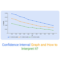
Learn what a confidence interval graph is, how to create it in Excel, and how to interpret results to make more reliable, data-driven decisions.
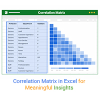
A correlation matrix in Excel helps identify relationships between variables. Learn how to create, read, and use it for effective data analysis.