Categories
VLOOKUP for Google Sheets? This powerful function transforms how users handle data in spreadsheets.
Imagine sifting through thousands of rows to find specific information – a tedious task that could take hours. VLOOKUP retrieves that data in seconds.
With over 3 billion users globally, Google Sheets has become essential to many businesses’ daily operations. Among its arsenal of functions, VLOOKUP stands out as a fan favorite. It’s the digital equivalent of a skilled assistant, swiftly locating and extracting information from vast datasets.


The function’s popularity stems from its versatility. From finance professionals consolidating reports to marketers creating dynamic dashboards, VLOOKUP’s applications are vast. It’s particularly useful for tasks like matching customer orders with product prices or pulling employee information for organizational charts.
However, VLOOKUP has limitations. It can only search vertically and return a single value at a time. Users often turn to advanced functions like QUERY for more complex data manipulations. Yet, VLOOKUP remains an indispensable tool for straightforward lookups and data retrieval in the Google Sheets ecosystem.
As businesses continue to rely on data-driven decision-making, mastering VLOOKUP for Google Sheets becomes increasingly valuable. It’s not merely about efficiency; it’s about empowering users to harness the full potential of their data.
Let’s see how to turn raw numbers into actionable insights using the VLOOKUP in Google Sheets.
First…
Definition: VLOOKUP in Google Sheets is a function that finds specific data in a table. It is abbreviated as “Vertical Lookup.”
This function searches for a value in the first column and returns it to the specified column and row.
VLOOKUP helps you to quickly retrieve information, like matching a product code with its price. It is ideal for large datasets where manual searching would be time-consuming. It’s a powerful tool for data organization and data analysis.
The VLOOKUP function in Google Sheets is a powerful tool for quickly searching and retrieving specific data from a table or dataset. Here’s why you should use it:
=VLOOKUP(search_key, range, index, [is_sorted])
VLOOKUP in Google Sheets is a handy tool. However, there are vital points to note for it to work smoothly. Let’s explore the five essentials.
VLOOKUP is your go-to function. Here’s a step-by-step guide on how to use it:
Prepare your data: Make sure your data is organized into columns.
Enter the VLOOKUP formula: Click on the cell where you want the result to appear. Type VLOOKUP formula.
This is the basic syntax: =VLOOKUP (lookup value, range, col index, [is sorted])
Where:
For example, if you’re looking up a product’s price from column A, type:
`=VLOOKUP (A2, A2:D10, 3, FALSE)`
Data analysts, unite. Your spreadsheets are rebelling. Numbers are multiplying faster than rabbits, and graphs are not making sense.
The solution? Data visualization. It turns mind-numbing digits into eye-catching stories.
But wait! Graphing data in Google Sheets feels like solving a Rubik’s Cube blindfolded. Its Google Sheets charts are often dull and uninspiring.
But fear not, data warriors; we have ChartExpo. With ChartExpo, your Scatter plot and other visuals don a tuxedo and tap dance across the screen. Insights pop like fireworks, and decision-makers stay awake during data presentations.
Who knew number crunching could be this fabulous?
Do not hesitate. Install ChartExpo now!
Let’s learn how to install ChartExpo in Google Sheets.
ChartExpo charts are available both in Google Sheets and Microsoft Excel. Please use the following CTAs to install the tool of your choice and create beautiful visualizations in a few clicks in your favorite tool.
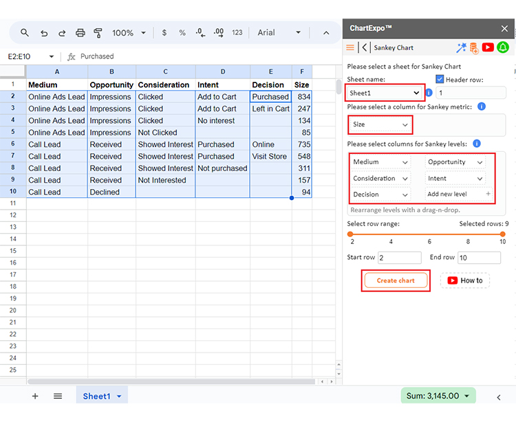
Let’s visualize and analyze the data below in Google Sheets using ChartExpo.
| Medium | Opportunity | Consideration | Intent | Decision | Size |
| Online Ads Lead | Impressions | Clicked | Add to Cart | Purchased | 834 |
| Online Ads Lead | Impressions | Clicked | Add to Cart | Left in Cart | 247 |
| Online Ads Lead | Impressions | Clicked | No interest | 134 | |
| Online Ads Lead | Impressions | Not Clicked | 85 | ||
| Call Lead | Received | Showed Interest | Purchased | Online | 735 |
| Call Lead | Received | Showed Interest | Purchased | Visit Store | 548 |
| Call Lead | Received | Showed Interest | Not purchased | 311 | |
| Call Lead | Received | Not Interested | 157 | ||
| Call Lead | Declined | 94 |


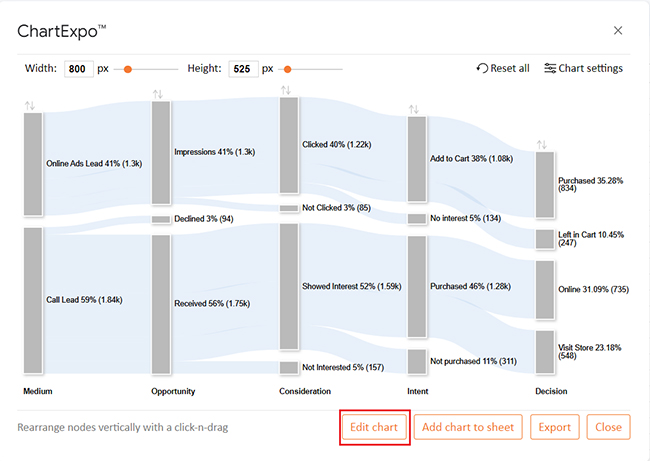
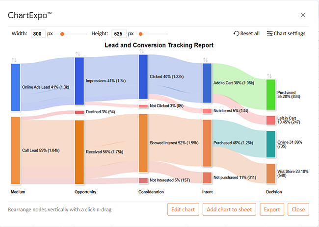
The following video will help you to create a Sankey Chart in Google Sheets.
VLOOKUP function in Google Sheets is a time-saver when managing datasets. It helps you quickly find and retrieve information with just a few clicks.
Here are the key benefits:
VLOOKUP in Google Sheets is a powerful tool, but using it effectively requires a few smart tips. Here are the top five tips to ensure smooth, accurate lookups:
Using VLOOKUP in Google Sheets is super helpful, but it works best when done right. Here are some best practices to get the most out of it:
To use VLOOKUP in Google Sheets, enter `=VLOOKUP(search_key, range, index, FALSE)` in a cell. This searches for the search key in the first column of the range. Then, it returns data from the specified index column in another sheet.
You can use VLOOKUP in Google Sheets to match survey responses with corresponding data. Enter `=VLOOKUP(response, range, column, FALSE)` to find specific answers and link them to categories or scores. This simplifies data analysis across different sheets.
VLOOKUP in Google Sheets helps organize data for multi-axis line charts by retrieving values from different sheets or tables. Use it to match and align specific data points. Then, plot the retrieved data on separate axes for a more precise comparison.
VLOOKUP in Google Sheets is a powerful function that helps you search for data. It simplifies the process of finding specific information in large datasets. With a few simple steps, VLOOKUP allows you to locate values based on a specific key.
The function scans a table and returns related data from other columns. It saves time by automating lookups instead of manually searching. This is especially useful for financial reports, inventories, and databases.
VLOOKUP is easy to use but requires proper setup. Your data must be organized, and you should use exact matches for precise results. Combining it with functions like `IFERROR` can improve the accuracy of your sheets.
It also offers flexibility. You can use it in various scenarios like matching IDs, prices, or product details. Moreover, it can be enhanced with other formulas for more advanced tasks.
In summary, VLOOKUP is a valuable tool for data management. It’s quick, efficient, and keeps data organized.
Start using it today with chartExpo for efficient data management and analysis.
Related Articles:
How much did you enjoy this article?


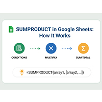
SUMPRODUCT in Google Sheets handles multi-condition calculations without extra columns. Master its syntax, uses, and errors. Read on!
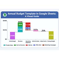
An annual budget template in Google Sheets organizes your yearly finances, tracks every dollar, and reveals spending patterns. Read on!
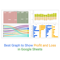
Learn the best graph to show profit and loss with practical examples and use cases. Discover how to visualize your business data, track trends, and make smarter financial decisions.