How to Transpose Data in Excel: A Step-by-Step Guide

How do you transpose data in Excel? Excel’s transpose function lets you easily move data from rows to columns and vice versa. This helps to save time and prevent annoyance.

This feature can completely change the game for anyone who has dealt with reorganizing rows and columns.

According to Microsoft, Excel is utilized by more than one billion individuals. This establishes it as a popular tool among businesses and professionals globally. Yet, many struggle with organizing data efficiently. That’s where learning how to transpose data in Excel comes in handy.

Say you’ve got a lengthy list in rows but need it displayed as columns, manually retyping everything isn’t an option. Transposing data allows you to rearrange your spreadsheet in seconds. This function can increase your productivity by 20%, according to a study by IDC.

The best part? You don’t need advanced Excel skills to use this function. With Excel’s flexibility, a few clicks can transform how you view and work with your data.

Why spend time on manual data entry when a quick transpose can do the job? Today, mastering these small yet powerful tools can make all the difference in staying efficient and accurate. Moreover, if you’re handling numbers daily, using transpose in Excel is a skill you’ll want in your toolbox.

Let’s get started.

Table of Contents:

1. What is Transpose Data in Excel?
2. What Does It Mean to Transpose Rows and Columns in Excel?
3. Why is Using Transpose Rows and Columns Important in Excel?
4. How to Transpose Data in Excel?
5. An Alternative Method to Transpose Values in Excel
6. How to Create a Visualization in Excel?
7. Tips for Using Transpose in Excel
8. Wrap Up

First…

What is Transpose Data in Excel?

Definition: Transpose data in Excel is a feature that lets you switch the orientation of your data. It converts rows into columns and columns into rows. This is useful when you need to rearrange information without manually retyping it.

Instead of reorganizing large data sets by hand, you can use the transpose function to save time. It ensures that your data remains accurate while being quickly reformatted to suit your needs. his feature is a great way to simplify your workflow.

What Does It Mean to Transpose Rows and Columns in Excel?

Definition: To transpose rows and columns in Excel means swapping their positions. Rows become columns, and columns turn into rows.

This is useful when your data is structured the wrong way. For example, if your headers are listed vertically but need to be horizontal, transposing fixes that.

You don’t have to manually move data, Excel’s transpose function handles it. This saves time and ensures the accuracy of your data while organizing it in the desired format.

Why is Using Transpose Rows and Columns Important in Excel?

Using transpose rows and columns in Excel can make a big difference in handling data. Organizing your information properly helps you work faster and with fewer mistakes.

Here’s why transposing data is important.

• Data organization: Transposing helps arrange your data in the most logical format, making it easier to manage and understand.
• Improved readability: Flipping rows into columns often makes data more readable. It allows you to present information more clearly.
• Efficient analysis: When data is properly structured, you can analyze it more quickly. This is especially helpful with large datasets.
• Presentation: Whether creating reports or sharing with others, transposing ensures your data looks professional and organized.
• Data comparison: Transposing makes it simpler to compare data side by side. You can quickly spot trends or inconsistencies.

How to Transpose Data in Excel?

Learning how to transpose data in Excel is simple and can save you time. Here’s a quick guide to help you switch your rows and columns with ease.

1. Select the data: Start by selecting the data you want to transpose. Highlight the entire range, including headers, if needed.
2. Copy the data: Once selected, copy the data by right-clicking and choosing “Copy” or using the shortcut Ctrl + C.
3. Choose the destination: Right-click the cell where you want the transposed data to appear. Go to “Paste Special” and check the “Transpose” option. Your data will instantly flip between rows and columns!

An Alternative Method to Transpose Values in Excel

Have you ever faced a situation where you needed to flip your data around in Excel? If copy-pasting doesn’t cut it, there are quick ways to move columns in Excel and transpose your rows and columns with just a few clicks!

Let’s explore them.

How to Transpose Rows and Columns Using Paste Options?

Need to switch up your data’s orientation? It’s easy!

1. Select the data you want to transpose, including any column or row labels.
2. Go to the “Home” tab.
3. Press “Ctrl” + “C” on your keyboard to copy the data.
4. Click on the new location where you want to paste your data. You can select a range of cells or just the top-right cell of your new data area.
5. Right-click the selected cell and choose “Paste Options” from the menu. Select the icon labeled “Transpose” when you hover over it.
6. Delete the original data. Your new table will maintain the desired layout and preserve any formatting from the original set, like colors or fonts.

How to Transpose Rows and Columns Using the Transpose Function?

Are you looking for a more dynamic way to transpose your data? Try the TRANSPOSE function. Here’s how to do it:

1. Determine the number of rows and columns needed for the transposed data. For example, let’s say your current table has five rows and eight columns. Your transposed table should have eight rows and five columns.
2. Select a range of cells that matches the required number of rows and columns for your transposed data.
3. Press the “F2” key to enter edit mode while keeping the range highlighted.
4. In the formula bar, type =TRANSPOSE, followed by the range of your original data in parentheses, like =TRANSPOSE(A1:G4) or =TRANSPOSE(B3:H7).
5. To apply the formula, press “Ctrl” + “Shift” + “Enter” (or just “Enter”, depending on your Excel version). This will save the changes and transpose your data.

How to Transpose Rows and Columns with Direct References?

Want to flip your data but keep everything linked? Using direct references is the way to go:

1. Click on an empty cell where you want to transpose your data and enter a reference followed by the cell location. For example, use “hh” followed by “B3” to reference cell B3.
2. In the cell below, enter the same reference and the next cell you want to transpose, like “hhB4”.
3. Select both cells, then use the drag feature to fill the desired range with your references.
4. Press “Ctrl” + “H” to open the “Find and Replace” menu.
5. In the “Find what” field, enter your chosen reference. In the “Replace” field, type the equal sign (“=”).
6. Click “Replace All” to complete the transposition of your data.

How to Transpose Rows and Columns with a Shortcut?

Are you looking for a quick way to swap rows and columns? Here’s a handy shortcut!

1. Highlight the range of cells you want to transpose.
2. Go to the “Data” tab at the top, then click “From Table”.
3. A pop-up window will show the selected date range. If it’s correct, click “OK”.
4. A new ribbon will appear. Select the “Transform” tab and then click on “Transpose”.

How to Transpose Data in Excel Without Zeros for Blanks?

Transposing data in Excel is a breeze. But what if you want to avoid having zeros where your blank cells should be? This is a common issue; luckily, there’s an easy fix. Follow these steps to transpose data without filling blanks with zeros.

1. Prepare your data: Start by organizing your data, ensuring any blank cells are where they need to be.
2. Replace zeros with blanks: If your data already has zeros where blanks should be, replace them with blanks. Use Excel’s “Find & Replace” tool (Ctrl + H) to clear those zeros quickly.
3. Copy the data: Highlight and copy the data you want to transpose. Right-click and select “Copy” or use Ctrl + C.
4. Select the destination cell: Choose the cell where you want the transposed data to appear. This will be the top-left corner of the new layout.
5. Transpose the data: Right-click the destination cell, go to “Paste Special,” and check the “Transpose” option. This will flip the rows and columns.
6. Verify the results: Double-check your transposed data to ensure the blanks are correctly in place and no zeros have appeared.

How to Create a Visualization in Excel?

Are you tired of flipping your data back and forth in Excel? Transposing data is just the beginning!

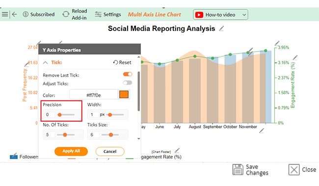
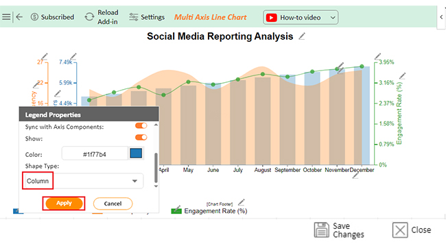
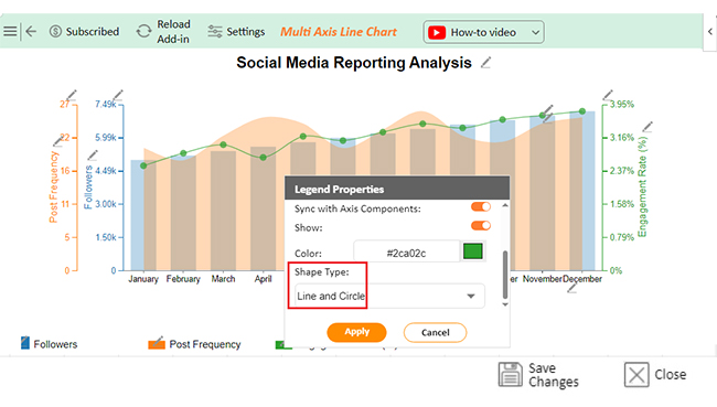
While Excel is great for crunching numbers, it often falls short when turning those numbers into compelling visuals. That’s where ChartExpo comes in. It’s a powerful tool that transforms static data into stunning charts and graphs, making your data analysis clear and engaging.

So, if you want to take your data visualization game to the next level, install ChartExpo.

But first…

Here are the top 5 charts in Excel:

Multi-Axis Line Chart

Sankey Chart

Likert Scale Chart

Comparison Bar Chart

Circular Org Chart

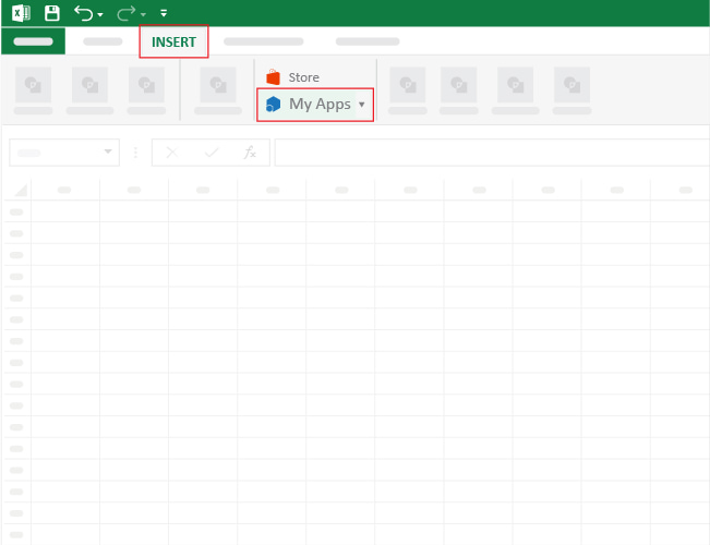
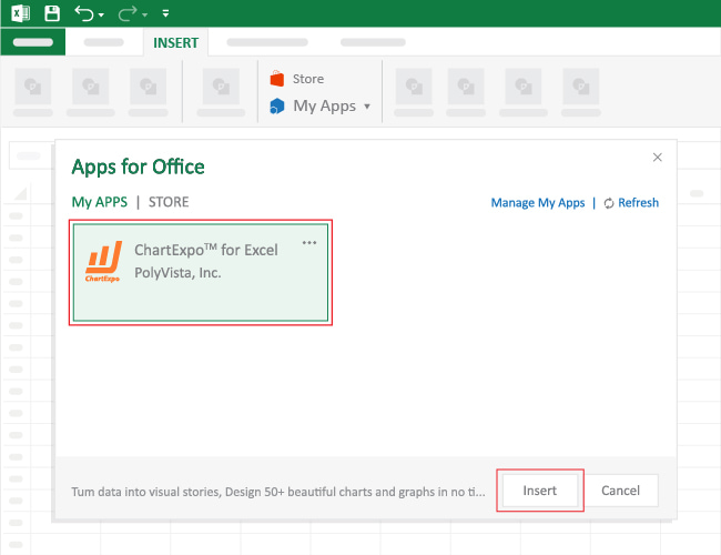
Let’s learn how to install ChartExpo in Excel.

1. Open your Excel application.
2. Open the worksheet and click the “Insert” menu.
3. You’ll see the “My Apps” option.
4. In the Office Add-ins window, click “Store” and search for ChartExpo on my Apps Store.
5. Click the “Add” button to install ChartExpo in your Excel.

ChartExpo charts are available both in Google Sheets and Microsoft Excel. Please use the following CTAs to install the tool of your choice and create beautiful visualizations with a few clicks in your favorite tool.

Example

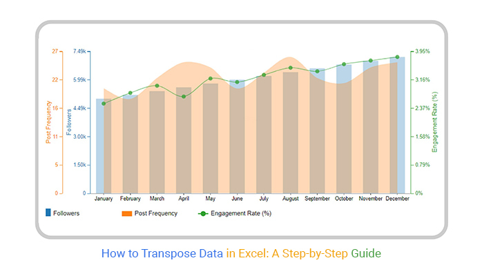
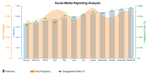
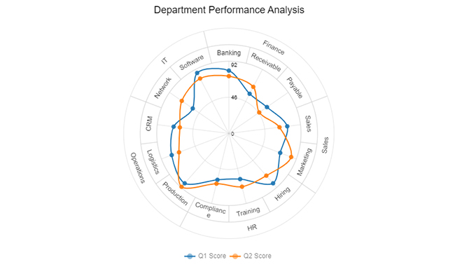
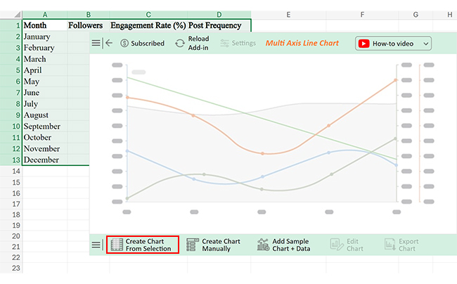
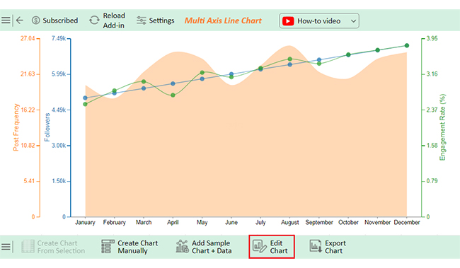
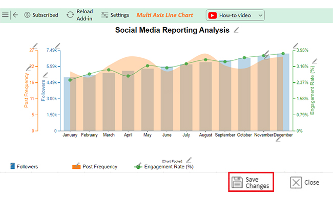
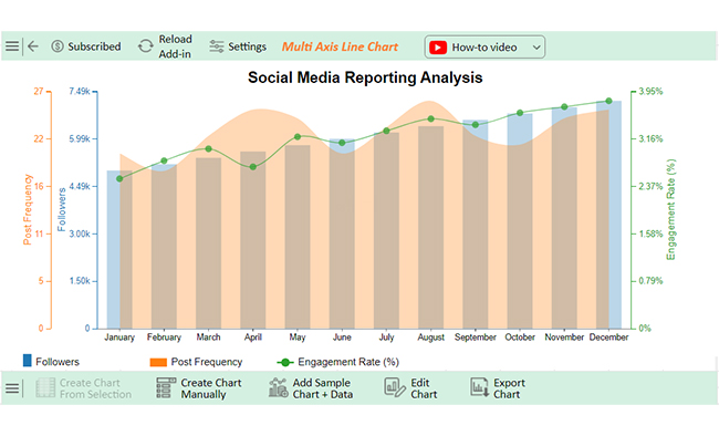
Let’s visualize the data below in Excel using ChartExpo and glean valuable insights.

Month	Followers	Engagement Rate (%)	Post Frequency
January	5000	2.5	20
February	5200	2.8	18
March	5400	3	22
April	5600	2.7	25
May	5800	3.2	24
June	6000	3.1	20
July	6200	3.3	23
August	6400	3.5	26
September	6600	3.4	22
October	6800	3.6	21
November	7000	3.7	24
December	7200	3.8	25

• To get started with ChartExpo, install ChartExpo in Excel.
• Now Click on My Apps from the INSERT menu.

• Choose ChartExpo from My Apps, then click Insert.

• Once it loads, scroll through the charts list to locate and choose the “Multi-Axis Line Chart”.

• Click the “Create Chart From Selection” button after selecting the data from the sheet, as shown.

• ChartExpo will generate the visualization below for you.

• Click on Settings and change the “Data Representation” as follows.

• If you want to add anything to the chart, click the Edit Chart button:
• Click the pencil icon next to the Chart Header to change the title.
• It will open the properties dialog. Under the Text section, you can add a heading in Line 1 and enable Show.
• Give the appropriate title of your chart and click the Apply button.

• You can add the sign of (%) with the Engagement Rate value:

• You can change the precision value to zero:

• Change the Legend shape of “Followers” to Column and click the “Apply” button.

• Change the Legend shape of “Engagement Rate” into a Line and Circle and click the “Apply” button.

• Click the “Save Changes” button to persist the changes made to the chart.

• Your final Multi Axis Line Chart will look like the one below.

Insights

• The follower count steadily increased throughout the year, reaching 7,200 by December.
• The engagement rate also improved, peaking at 3.8%.
• Post frequency fluctuated but stayed fairly consistent, reflecting strong audience growth and engagement strategies over the months.

Tips for Using Transpose in Excel

Before you jump into transposing data in Excel, there are some key things to keep in mind. These tips will help you keep your data clean and organized.

• Check data size: Ensure your data isn’t too large for Excel to handle. The transpose function may slow down or cause errors if your data set is massive.
• Use Paste Special: The “Paste Special” option lets you transpose your data instantly. Just copy your data, right-click, and select “Transpose” under Paste Special.
• Clear old data: After transposing, you’ll want to clear the old data to avoid confusion. This keeps your spreadsheet tidy and easy to follow.
• Copy vs. cut: When transposing, consider whether to copy or cut. Copying leaves the original data intact while cutting moves it. Use the option that best fits your needs.
• Formula adjustment: Be aware that transposing data can affect your formulas. Excel may change references when you transpose them. Double-check your formulas afterward to ensure everything works correctly.

FAQs

How do you transpose data in Excel with formulas?

Use the TRANSPOSE function:

• Select the destination cells.
• Enter =TRANSPOSE(A1) (adjust for your range).
• Press Ctrl + Shift + Enter to apply as an array formula.
• The data will update with the source automatically.

How do you TRANSPOSE multiple rows into one column?

• Highlight the rows you want to transpose.
• Copy the data (Ctrl + C).
• Right-click the destination cell.
• Select Paste Special and check the Transpose
• The rows will now appear as a single column.

Wrap Up

Transposing data in Excel is a useful skill. It helps you switch rows and columns effortlessly.

You can use various methods based on your needs. The Paste Special option is quick for static data. It’s perfect when you need a simple flip without updates.

The TRANSPOSE function offers a dynamic solution. It links the original and transposed data. Any changes made to the source are reflected in the transposed table. This method is ideal for data that updates frequently.

Direct references also work well for transposition. You manually set up references to the original cells. Then, you replace those references with formulas. This approach is useful for more control over your data.

Shortcuts can save time, too. A quick “Copy” and “Transpose” paste can do the trick. They’re effective for simple, one-time tasks.

While Excel handles data manipulation well, it has limits. Visual representation can be challenging without additional tools. Using ChartExpo will enhance your data analysis.

Do not hesitate.

Install ChartExpo to transform complex data into clear, interactive visuals.