Categories
Spreadsheets often demand calculations that go beyond basic addition or subtraction. SUMPRODUCT in Google Sheets is a built-in function that multiplies values across ranges and returns their sum in one step, eliminating the need for helper columns or stacked formulas.
Whether the goal is sales totals, weighted scores, or conditional summaries, this function covers it.
This blog covers everything from the syntax and basic usage to multiple-criteria filtering, real-world examples, and common errors. By the end, you will know how to apply SUMPRODUCT to your own datasets and extract the results you need.
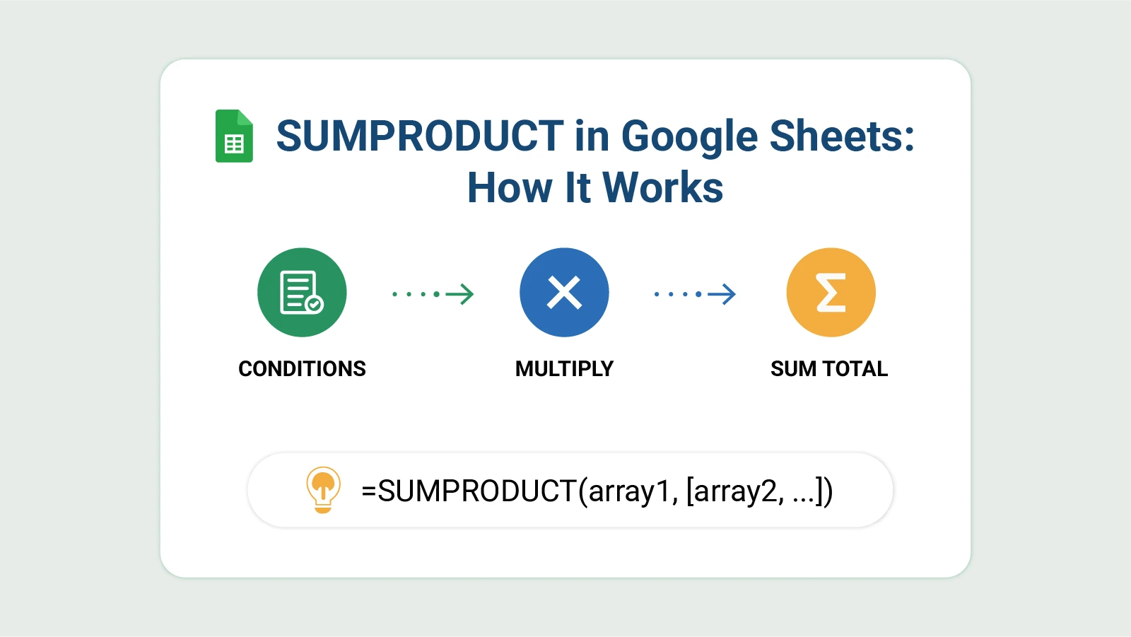
Definition: SUMPRODUCT in Google Sheets is a built-in function that takes two or more arrays, multiplies their corresponding values row by row, and returns a single total. Rather than treating multiplication and addition as separate operations, it combines them into one formula, which reduces clutter in any spreadsheet.
The formula handles arrays, ranges, and conditional logic, making Google Sheet SUMPRODUCT a practical tool for business reports, financial models, and sales tracking.
Where the SUM function is limited to adding a column of numbers, this function can work across multiple columns at once. It also accepts conditions and logical expressions, so calculations can target only the rows that meet certain criteria. As a result, a single formula can replace several nested IF statements.
Routine spreadsheet work often requires logic that a single SUM cannot handle.
Several factors explain why this function is relied on across industries:
The SUMPRODUCT formula in Google Sheets identifies values in the same position across each array provided, multiplies them together, and then totals all the resulting products. Any numeric data organized in rows is a candidate for this approach.
SUMPRODUCT(array1, [array2, array3, …])
All arrays supplied to the function must contain an equal number of cells. When given several arrays, each row is evaluated independently before the total is calculated.
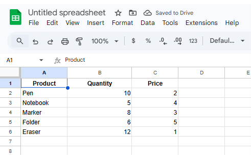
Using Google Sheet SUMPRODUCT is straightforward when data is laid out in columns. Follow these steps to apply the function correctly.
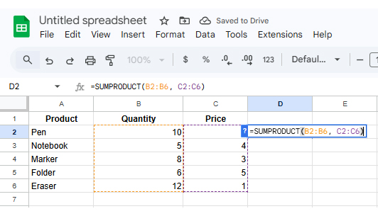
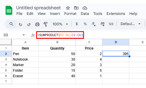
Enter your data in columns so that each row represents one record. Make sure the Quantity and Price columns have the same number of rows; SUMPRODUCT will return an error.
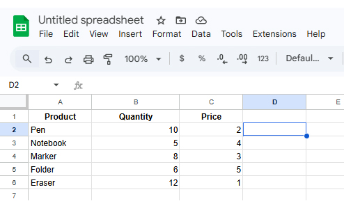
Click on an empty cell where you want the final total.
Example: click on cell D2 to display the result.
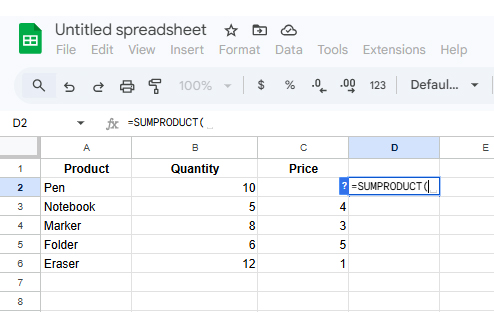
Type the formula starting with = and then write SUMPRODUCT.
=SUMPRODUCT(
Do not press Enter yet.
Select the Quantity range first, then the Price range.
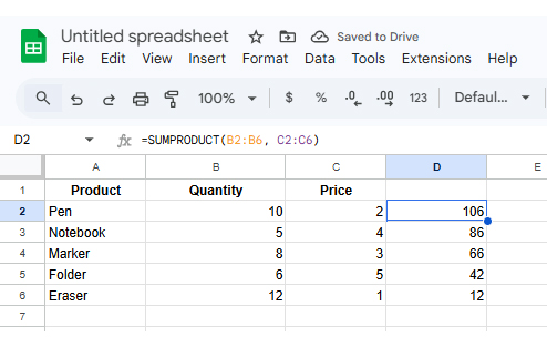
=SUMPRODUCT(B2:B6, C2:C6)
The function will multiply each row and then add all results.
If you want totals for specific items, you can add conditions.
Press Enter, and Google Sheets will return the total sales value.
For horizontal datasets, consider combining this approach with Google Sheets HLOOKUP when row-based lookups are also needed.
The real power of SUMPRODUCT in Google Sheets expands what a single formula can accomplish. Rather than filtering a dataset manually, conditions are embedded directly into the expression, so only matching rows contribute to the result.
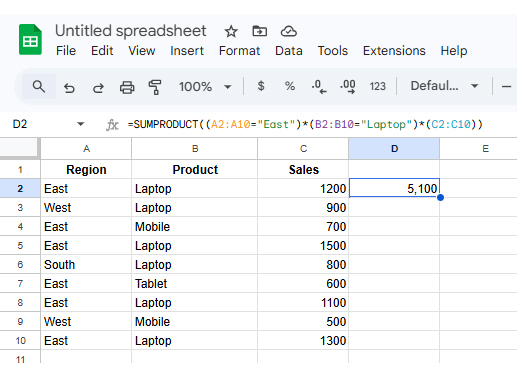
Example with criteria:
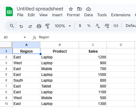
Enter the following data in your sheet.
Click on an empty cell where you want the result.
Example: select cell E2.
Type the formula:
=SUMPRODUCT((A2:A10=”East”)*(B2:B10=”Laptop”)*(C2:C10)
Explanation:
Only rows where both conditions are TRUE will be included.
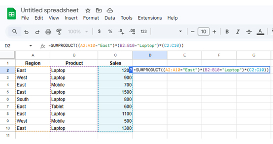
After pressing Enter, Google Sheets will return:
This technique removes the need to use the Google Sheets query function when the goal is filtering by field values inside a formula.
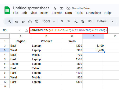
Filtering by condition ranks among the most frequent uses for SUMPRODUCT in Google Sheets. The formula accepts comparison operators directly, so results are scoped to rows that pass the test without any extra filtering layer.
The example below uses the same dataset from the previous section (Region, Product, Sales) and applies a different condition to calculate the total for specific rows only.
=SUMPRODUCT((A2:A10=”East”)*(B2:B10>700)*(C2:C10))
The first condition checks Region = East, and the second checks Sales > 700, so only matching rows are included in the final total.
This approach fits naturally into any workflow built around structured data, particularly when categories are stored in separate fields as part of how to group columns in Google Sheets.
Three scenarios show the function in practice.
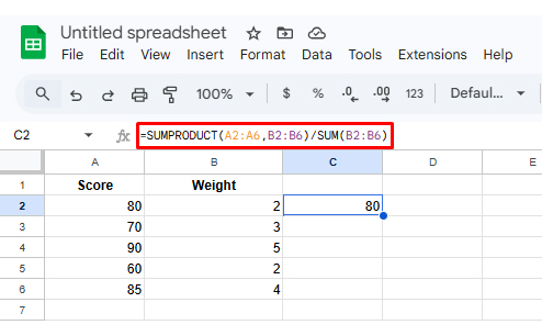
Applied when scores, ratings, or marks carry different levels of importance and a simple average would misrepresent the result.
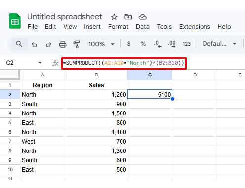
Used to total revenue for a single region or category by embedding a condition, with no need to filter the dataset first.
Used to compute total stock value by multiplying units on hand by unit cost for each item and summing the products.
These scenarios are directly relevant when building reports that also rely on averages in Google Sheets for summary calculations.
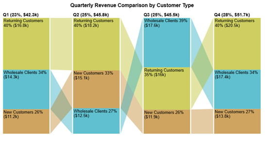
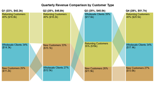
The quarterly revenue comparison by customer type chart shows returning customers lead revenue in most quarters, with Q4 recording the top overall total.
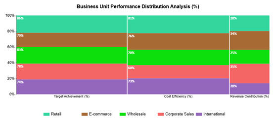
The business unit performance distribution analysis shows the percentage share each unit holds across performance metrics, all derived from SUMPRODUCT calculations.
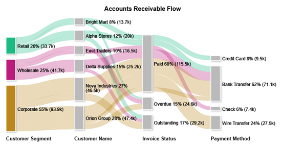
The accounts receivable flow chart maps revenue distribution across categories and channels, drawing on SUMPRODUCT for the multi-level breakdown.
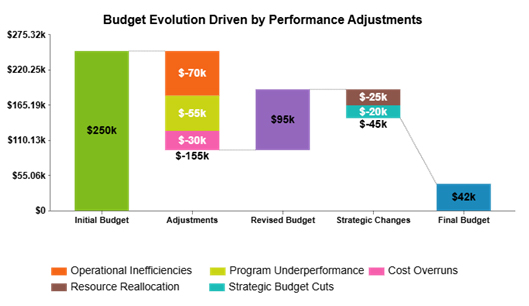
The budget evolution driven by performance adjustments chart shows how individual revenue and expense items combine to form the final total, using SUMPRODUCT for multi-category financial tracking.
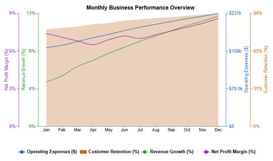
The monthly business performance overview chart tracks expenses, revenue, retention, and profit month by month, using SUMPRODUCT to support the underlying performance analysis.
Analyzing SUMPRODUCT output in Google Sheets allows you to evaluate weighted calculations, segment contributions, and uncover deeper insights from structured datasets.
Since SUMPRODUCT combines arrays to return aggregated results, understanding its output is essential for accurate financial and performance analysis.
Start by identifying what the SUMPRODUCT formula is calculating—whether it’s weighted revenue, cost allocation, or performance scoring.
Review the arrays used in the formula to understand how each variable contributes to the final output.
Ensure all input ranges are aligned, consistent, and free from errors, as mismatched arrays can distort results.
Divide the result into meaningful categories (e.g., customer types, quarters, or regions) to interpret contributions clearly.
Analyze how values change across different segments to identify growth patterns, high-performing areas, or inefficiencies.
Convert SUMPRODUCT insights into visualizations such as comparison charts or flow diagrams. For advanced and interactive visuals, use ChartExpo to simplify complex relationships.
Include a final visualization to highlight how different segments contribute to the overall result. For example, the image below shows how customer types contribute to quarterly revenue, helping you interpret SUMPRODUCT-driven insights more effectively.
Small mistakes inside a formula can generate incorrect totals or trigger errors.
Watch for these common problems:
Choose SUMPRODUCT in Google Sheets when a calculation involves multiplying values before totaling them, or when more than one condition must be met. SUM handles straightforward column addition, but it cannot apply criteria or work across multiple arrays at once.
It pairs the values in matching positions across two or more arrays, multiplies each pair, and returns the total of all those products. The SUMPRODUCT formula in Google Sheets is commonly applied to weighted averages, filtered totals, and financial reporting.
Yes. The function is built to process arrays and ranges together, which is what makes Google Sheet SUMPRODUCT well-suited for datasets where several columns interact in a single calculation. It also accepts logical expressions, so rows can be filtered by condition without a separate formula.
Mastering SUMPRODUCT in Google Sheets removes the ceiling on what a single formula can accomplish. The function handles array multiplication, conditional filtering, and weighted totals without requiring helper columns or nested IF statements, which keeps spreadsheets clean and makes every calculation easy to trace.
The skills covered here, from basic syntax to multi-criteria filtering and error diagnosis, apply directly to the kinds of datasets most analysts work with every day. Build these techniques into your workflow, and both accuracy and reporting efficiency will improve as a result.
How much did you enjoy this article?


An annual budget template in Google Sheets organizes your yearly finances, tracks every dollar, and reveals spending patterns. Read on!
Learn the best graph to show profit and loss with practical examples and use cases. Discover how to visualize your business data, track trends, and make smarter financial decisions.
Learn how to create a Sankey diagram in Google Sheets to visualize flows such as customer journeys, energy transfers, and cash movements for deeper insights and analysis.